Data Analysis on Wine Data Sets with R
We will apply some methods for supervised and unsupervised analysis to two datasets. This two datasets are related to red and white variants of the Portuguese vinho verde wine and are available at UCI ML repository.
Our goal is to characterize the relationship between wine quality and its analytical characteristics.
The output variable is a note between 0 (the worst) and 10 (the best) determined by expert evaluation. It can be considered as discrete categories so that this problem can be formulated as classification or regression.
We will develop models of wine quality for each of the wine variant to determine whether quality of red and white wine is influenced predominantly by the same or different analytical properties.
At the end of this tutorial we will combine analytical data and look for any well defined clusters.
1: Data Summary
First, we load the required librairies and data sets.
library(leaps)
library(ggplot2)
library(reshape2)
library(MASS)
library(ggcorrplot)
library(plotmo)

whiteDat = read.table("winequality-white.csv", sep = ";", header = T)
redDat = read.table("winequality-red.csv", sep = ";", header = T)
Then I create a shortcut function to sort the dataframe columns by the absolute value of their correlation with the outcome.
sortByCorr = function(dataset, refColName) {
  # Sort the dataframe columns by the absolute value of their correlation with
  # a given column
  #
  # Args:
  #   dataset: A vector, matrix, or data frame to sort
  #   refColName: The name of the reference colum for the correlation
  #
  # Returns:
  #   The sorted dataframe
  refColIdx = grep(refColName, colnames(dataset))
  corrTmp = cor(dataset)[, refColIdx]
  corrTmp[order(abs(corrTmp), decreasing = TRUE)]

  dataset[, order(abs(corrTmp), decreasing = TRUE)]
}
1.1: White wine data
1.1.a: Summary
dim(whiteDat)
## [1] 4898 12sapply(whiteDat, class)
##        fixed.acidity     volatile.acidity          citric.acid
##            "numeric"            "numeric"            "numeric"
##       residual.sugar            chlorides  free.sulfur.dioxide
##            "numeric"            "numeric"            "numeric"
## total.sulfur.dioxide              density                   pH
##            "numeric"            "numeric"            "numeric"
##            sulphates              alcohol              quality
##            "numeric"            "numeric"            "integer"
# We take a look at the data distribution:
head(whiteDat)
##   fixed.acidity volatile.acidity citric.acid residual.sugar chlorides
## 1           7.0             0.27        0.36           20.7     0.045
## 2           6.3             0.30        0.34            1.6     0.049
## 3           8.1             0.28        0.40            6.9     0.050
## 4           7.2             0.23        0.32            8.5     0.058
## 5           7.2             0.23        0.32            8.5     0.058
## 6           8.1             0.28        0.40            6.9     0.050
##   free.sulfur.dioxide total.sulfur.dioxide density   pH sulphates alcohol
## 1                  45                  170  1.0010 3.00      0.45     8.8
## 2                  14                  132  0.9940 3.30      0.49     9.5
## 3                  30                   97  0.9951 3.26      0.44    10.1
## 4                  47                  186  0.9956 3.19      0.40     9.9
## 5                  47                  186  0.9956 3.19      0.40     9.9
## 6                  30                   97  0.9951 3.26      0.44    10.1
##   quality
## 1       6
## 2       6
## 3       6
## 4       6
## 5       6
## 6       6
# Get some metrics about the variables
summary(whiteDat)
##  fixed.acidity    volatile.acidity  citric.acid     residual.sugar
##  Min.   : 3.800   Min.   :0.0800   Min.   :0.0000   Min.   : 0.600
##  1st Qu.: 6.300   1st Qu.:0.2100   1st Qu.:0.2700   1st Qu.: 1.700
##  Median : 6.800   Median :0.2600   Median :0.3200   Median : 5.200
##  Mean   : 6.855   Mean   :0.2782   Mean   :0.3342   Mean   : 6.391
##  3rd Qu.: 7.300   3rd Qu.:0.3200   3rd Qu.:0.3900   3rd Qu.: 9.900
##  Max.   :14.200   Max.   :1.1000   Max.   :1.6600   Max.   :65.800
##    chlorides       free.sulfur.dioxide total.sulfur.dioxide
##  Min.   :0.00900   Min.   :  2.00      Min.   :  9.0
##  1st Qu.:0.03600   1st Qu.: 23.00      1st Qu.:108.0
##  Median :0.04300   Median : 34.00      Median :134.0
##  Mean   :0.04577   Mean   : 35.31      Mean   :138.4
##  3rd Qu.:0.05000   3rd Qu.: 46.00      3rd Qu.:167.0
##  Max.   :0.34600   Max.   :289.00      Max.   :440.0
##     density             pH          sulphates         alcohol
##  Min.   :0.9871   Min.   :2.720   Min.   :0.2200   Min.   : 8.00
##  1st Qu.:0.9917   1st Qu.:3.090   1st Qu.:0.4100   1st Qu.: 9.50
##  Median :0.9937   Median :3.180   Median :0.4700   Median :10.40
##  Mean   :0.9940   Mean   :3.188   Mean   :0.4898   Mean   :10.51
##  3rd Qu.:0.9961   3rd Qu.:3.280   3rd Qu.:0.5500   3rd Qu.:11.40
##  Max.   :1.0390   Max.   :3.820   Max.   :1.0800   Max.   :14.20
##     quality
##  Min.   :3.000
##  1st Qu.:5.000
##  Median :6.000
##  Mean   :5.878
##  3rd Qu.:6.000
##  Max.   :9.000
The white wine dataset has 4898 observations, 11 predictors and 1 outcome (quality). All of the predictors are numeric values, outcomes are integer.
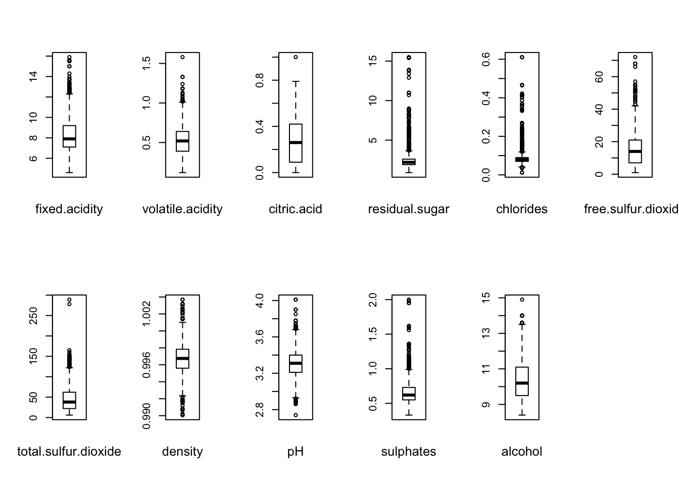
The summary stats shows that most of the variables has wide range compared to the IQR, which may indicate spread in the data and the presence of outliers.
We investigate further by producing boxplots for each of the variables:
oldpar = par(mfrow = c(2,6))
for ( i in 1:11 ) {
  boxplot(whiteDat[[i]])
  mtext(names(whiteDat)[i], cex = 0.8, side = 1, line = 2)
}
par(oldpar)
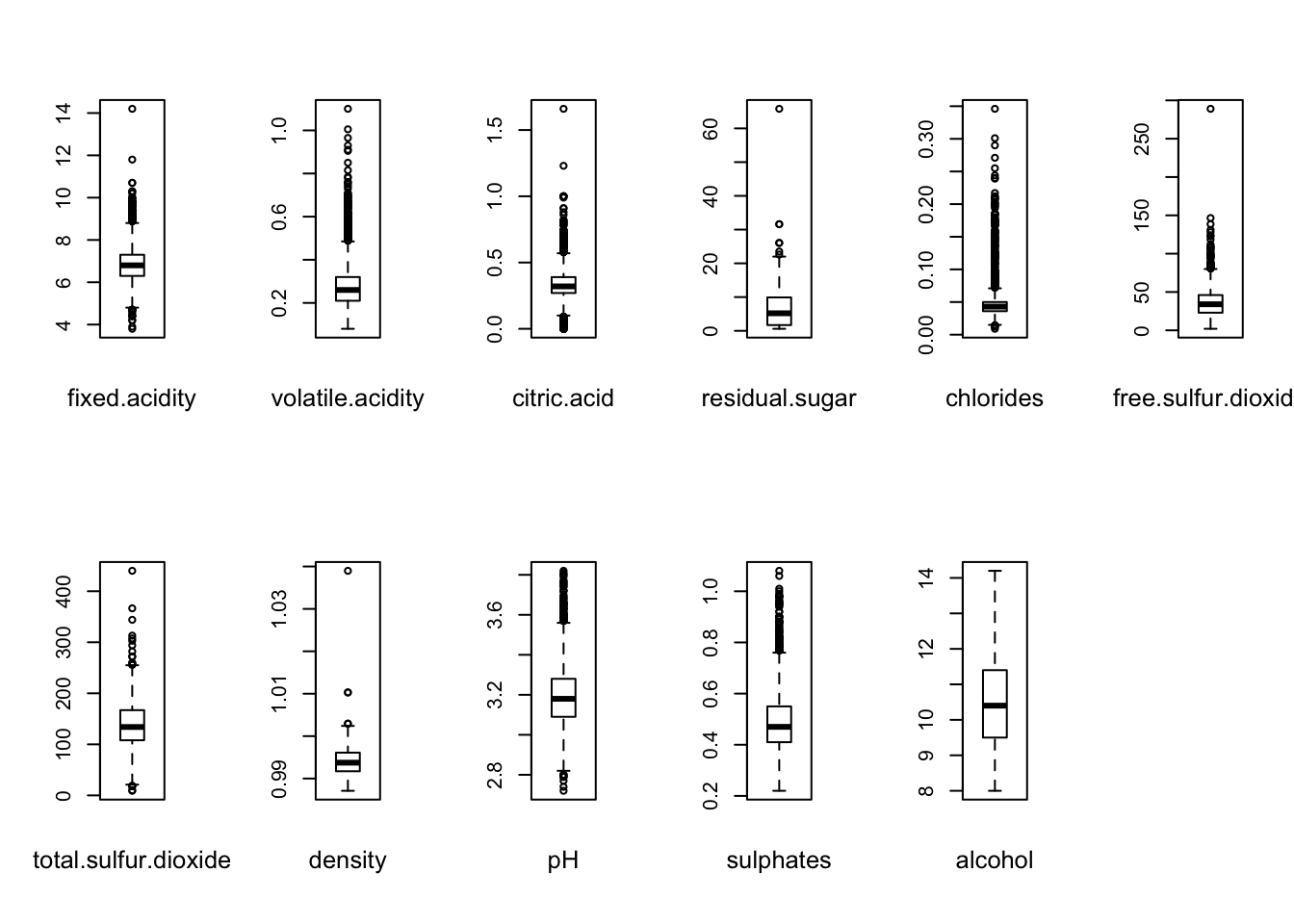
It demonstrate that all variables, except alcohol contains outliers.
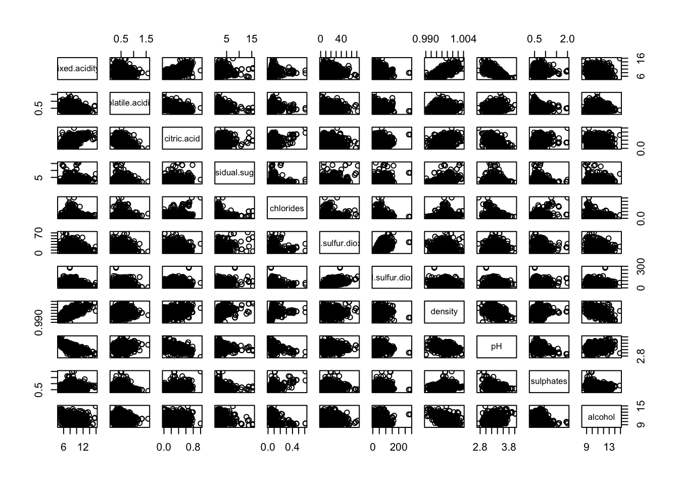
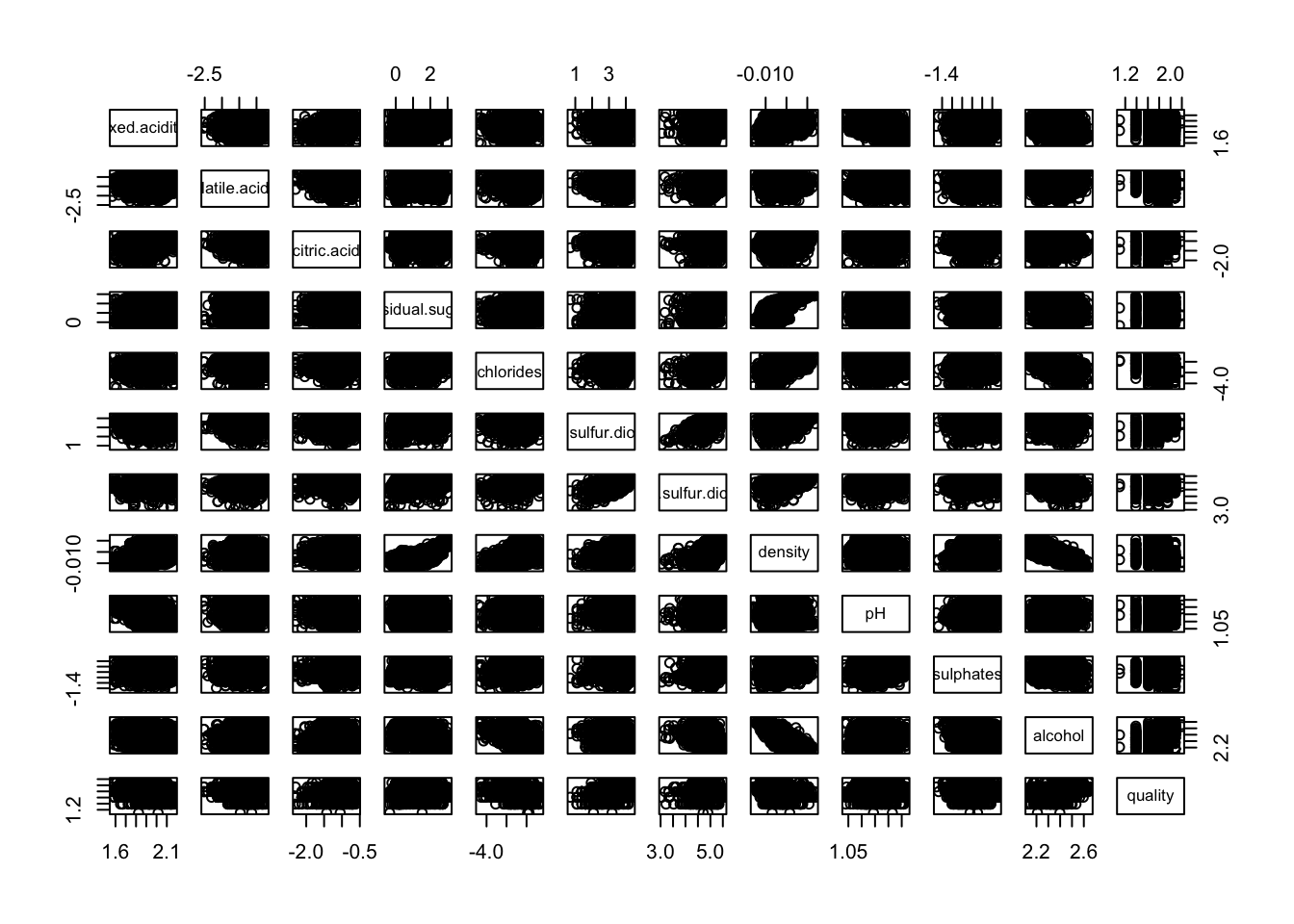
We now use a scatter plot matrix to get an insight on the outliers locations:
pairs(whiteDat[, -grep("quality", colnames(whiteDat))])
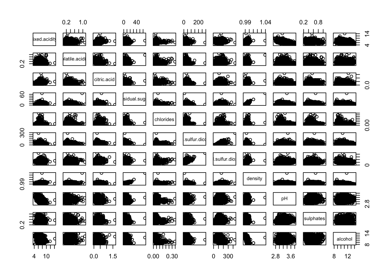
We see that outliers seems to be on the higher end.
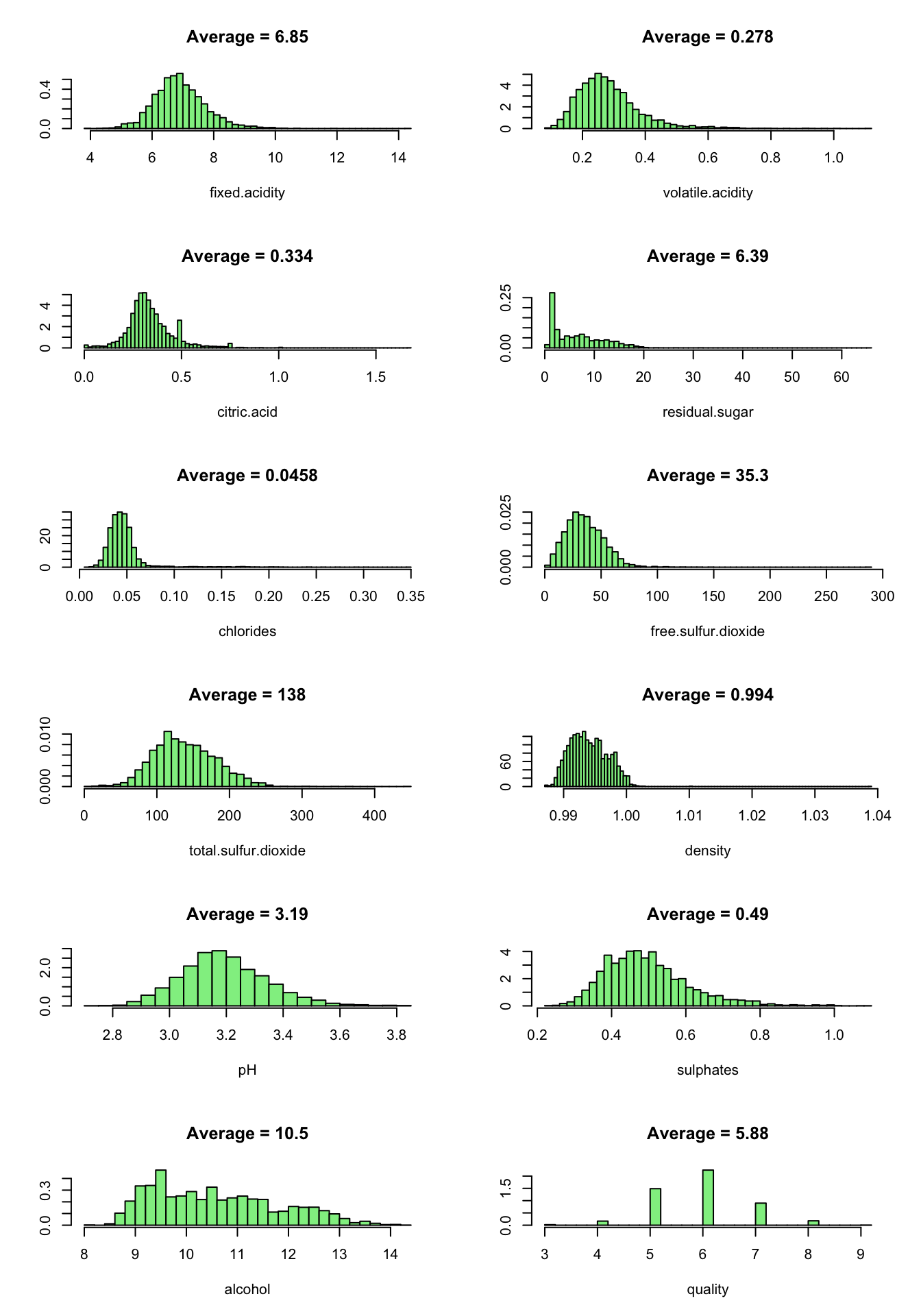
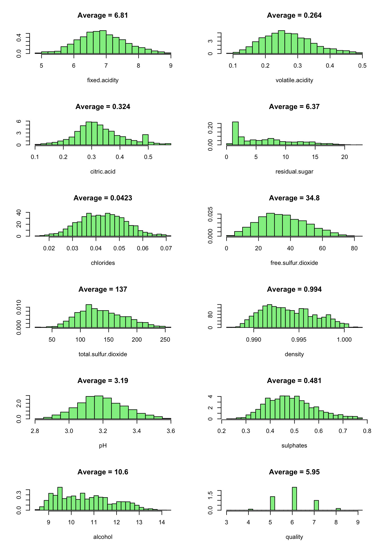
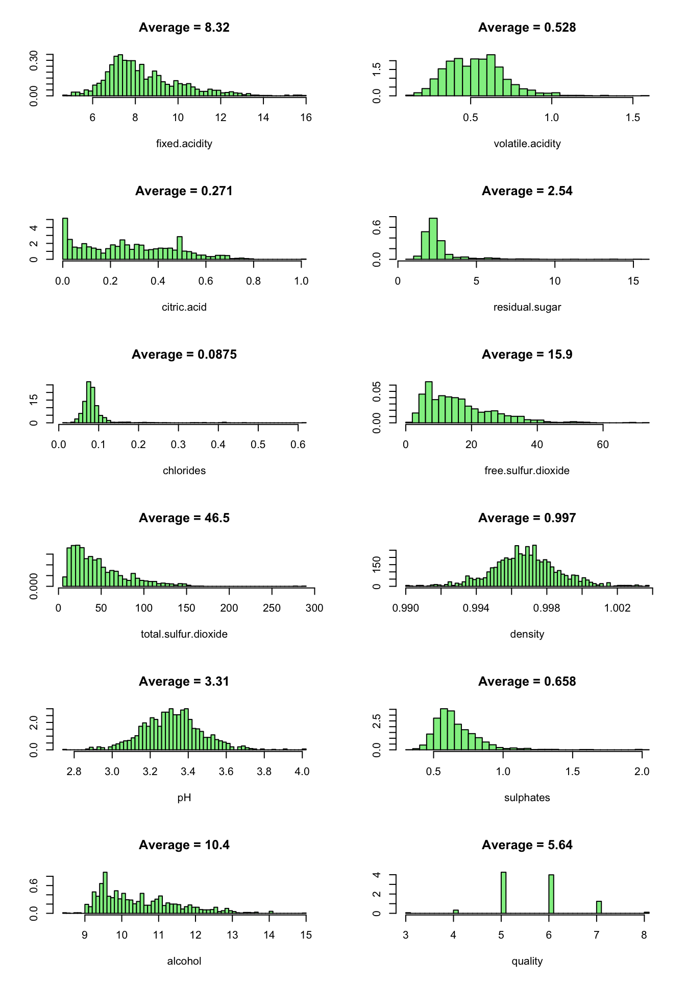
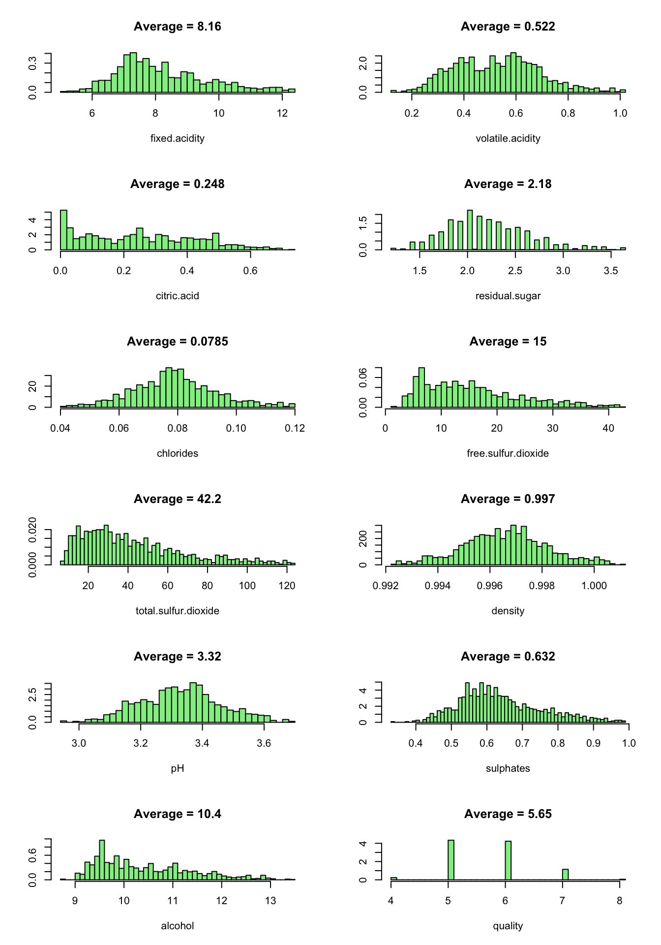
Now we look at the predictor values distribution:
oldpar = par(mfrow = c(6,2))
for ( i in 1:12 ) {
  truehist(whiteDat[[i]], xlab = names(whiteDat)[i], col = 'lightgreen', main = paste("Average =", signif(mean(whiteDat[[i]]),3)))
}
par(oldpar)
We note that all the variables has positively skewed distributions except quality which is normally distributed. citric.acide show a peak at the lower end.
1.1.b: Outlier detection
For each variables, we consider observations that lie outside 1.5 * IQR as outliers.
outliers = c()
for ( i in 1:11 ) {
  stats = boxplot.stats(whiteDat[[i]])$stats
  bottom_outlier_rows = which(whiteDat[[i]] < stats[1])
  top_outlier_rows = which(whiteDat[[i]] > stats[5])
  outliers = c(outliers , top_outlier_rows[ !top_outlier_rows %in% outliers ] )
  outliers = c(outliers , bottom_outlier_rows[ !bottom_outlier_rows %in% outliers ] )
}
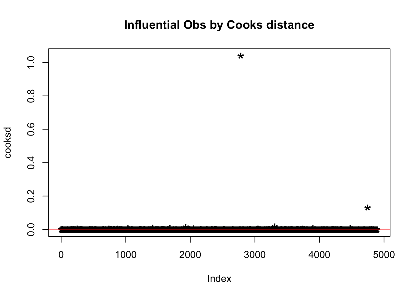
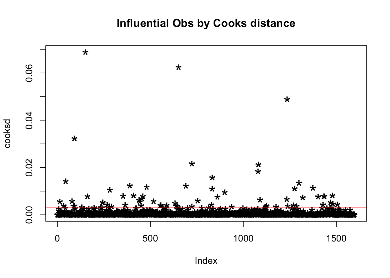
We use the Cook’s ditance to detect influential observations.
mod = lm(quality ~ ., data = whiteDat)
cooksd = cooks.distance(mod)
plot(cooksd, pch = "*", cex = 2, main = "Influential Obs by Cooks distance")
abline(h = 4*mean(cooksd, na.rm = T), col = "red")
head(whiteDat[cooksd > 4 * mean(cooksd, na.rm=T), ])
##     fixed.acidity volatile.acidity citric.acid residual.sugar chlorides
## 18            6.2             0.66        0.48            1.2     0.029
## 21            6.2             0.66        0.48            1.2     0.029
## 99            9.8             0.36        0.46           10.5     0.038
## 251           5.9             0.21        0.28            4.6     0.053
## 252           8.5             0.26        0.21           16.2     0.074
## 254           5.8             0.24        0.44            3.5     0.029
##     free.sulfur.dioxide total.sulfur.dioxide density   pH sulphates
## 18                   29                   75  0.9892 3.33      0.39
## 21                   29                   75  0.9892 3.33      0.39
## 99                    4                   83  0.9956 2.89      0.30
## 251                  40                  199  0.9964 3.72      0.70
## 252                  41                  197  0.9980 3.02      0.50
## 254                   5                  109  0.9913 3.53      0.43
##     alcohol quality
## 18     12.8       8
## 21     12.8       8
## 99     10.1       4
## 251    10.0       4
## 252     9.8       3
## 254    11.7       3
By looking at each row we can find out why it is influential:
- Row 99 and 252 have very high residual.sugar.
- Row 18 and 21 have very high free.sulfur.dioxide.
- Row 251 have very high sulphates.
- Row 254 and 99 have very low free.sulfur.dioxide.
We remove all the ouliers in our list from the dataset and create a new set of histograms:
coutliers = as.numeric(rownames(whiteDat[cooksd > 4 * mean(cooksd, na.rm=T), ]))
outliers = c(outliers , coutliers[ !coutliers %in% outliers ] )

cleanWhiteDat = whiteDat[-outliers, ]
oldpar = par(mfrow=c(6,2))
for ( i in 1:12 ) {
  truehist(cleanWhiteDat[[i]], xlab = names(cleanWhiteDat)[i], col = 'lightgreen', main = paste("Average =", signif(mean(cleanWhiteDat[[i]]),3)))
}
par(oldpar)
By removing the outliers, the dataset size reduced to 3999 observations.
Now, the variables are approximatly normaly distributed, except for residual.sugar which is unimodal and skewed to the right. This could be an interesting fact for further analysis.
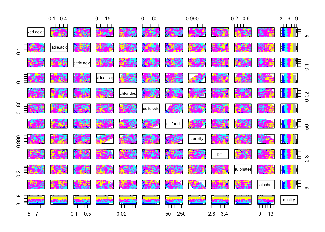
We now use a scatterplot matrice to roughly determine if there is a linear correlation between our variables:
pairs(cleanWhiteDat, col = cleanWhiteDat$quality, pch = cleanWhiteDat$quality)
pairs(cleanWhiteDat[,c(7, 8, 10, 11)], col = cleanWhiteDat$quality, pch = cleanWhiteDat$quality)
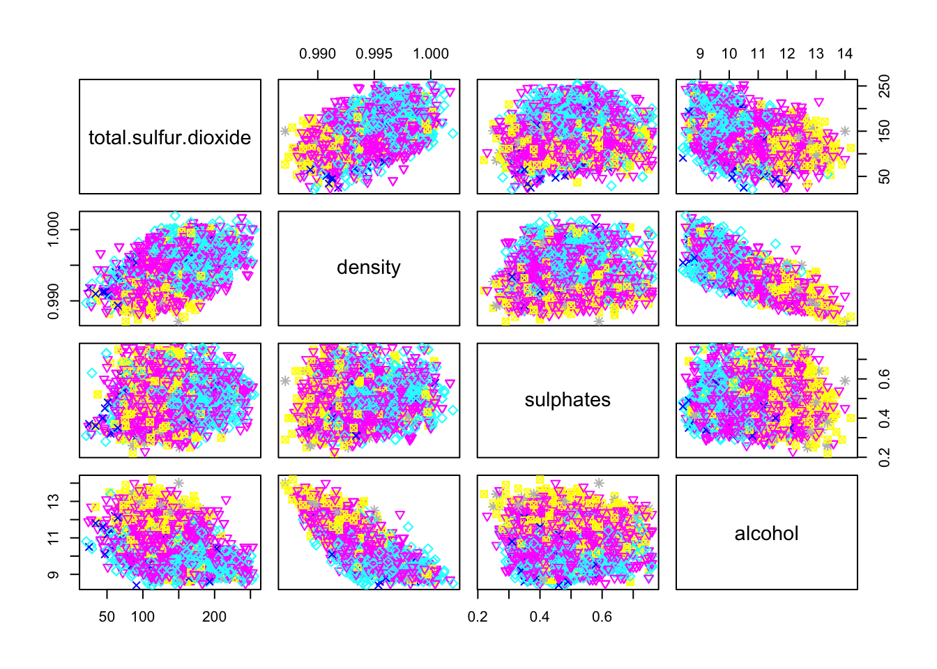
Only residual.sugar/density and density/alcohol pairs seems to have a linear correlation.
We note a trend with the alcohol variable: higher the alcohol value is, better is the quality.
In the oposite, it seems like the lowest the density, the better the quality.
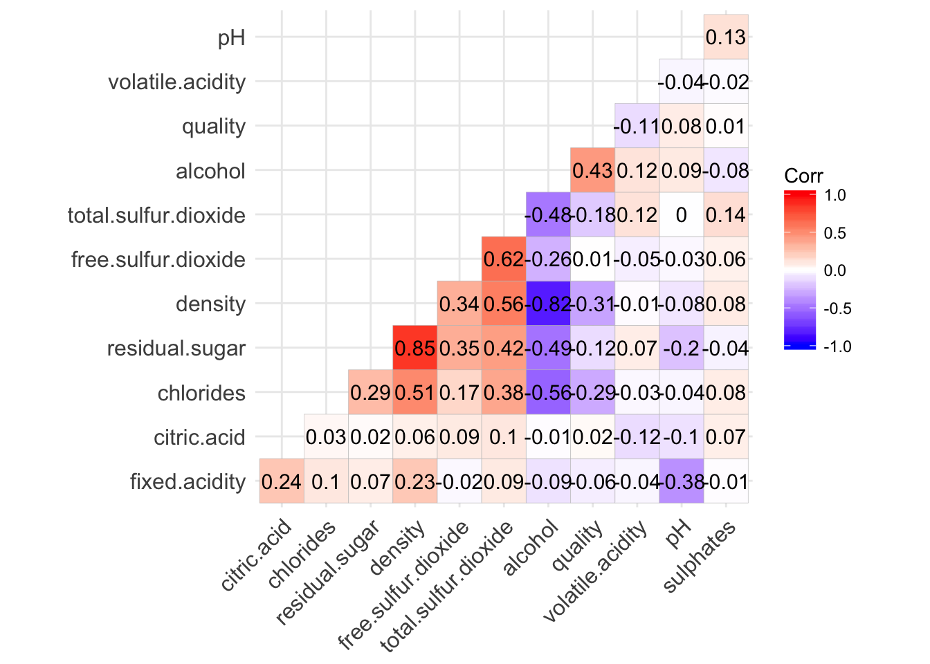
1.1.c: Correlation
The following correlation matrix confirm the strong correlation between residual.sugar/density and density/alcohol. It also confirm that alcohol is the variable with the highest correlation with quality. At a lower level, density and chlorides also have a significant correlation with quality.
ggcorrplot(cor(cleanWhiteDat), hc.order = TRUE, type = "lower", lab = TRUE, insig = "blank")
colnames(sortByCorr(dataset = cleanWhiteDat, refColName = 'quality'))
##  [1] "quality"              "alcohol"              "density"
##  [4] "chlorides"            "total.sulfur.dioxide" "residual.sugar"
##  [7] "volatile.acidity"     "pH"                   "fixed.acidity"
## [10] "citric.acid"          "sulphates"            "free.sulfur.dioxide"
1.2 Red wine data
We apply the same procedure to the red wine dataset.
1.2.a: Summary
dim(whiteDat)
## [1] 4898 12sapply(redDat, class)
##        fixed.acidity     volatile.acidity          citric.acid
##            "numeric"            "numeric"            "numeric"
##       residual.sugar            chlorides  free.sulfur.dioxide
##            "numeric"            "numeric"            "numeric"
## total.sulfur.dioxide              density                   pH
##            "numeric"            "numeric"            "numeric"
##            sulphates              alcohol              quality
##            "numeric"            "numeric"            "integer"
# We take a look at the data distribution:
head(redDat)
##   fixed.acidity volatile.acidity citric.acid residual.sugar chlorides
## 1           7.4             0.70        0.00            1.9     0.076
## 2           7.8             0.88        0.00            2.6     0.098
## 3           7.8             0.76        0.04            2.3     0.092
## 4          11.2             0.28        0.56            1.9     0.075
## 5           7.4             0.70        0.00            1.9     0.076
## 6           7.4             0.66        0.00            1.8     0.075
##   free.sulfur.dioxide total.sulfur.dioxide density   pH sulphates alcohol
## 1                  11                   34  0.9978 3.51      0.56     9.4
## 2                  25                   67  0.9968 3.20      0.68     9.8
## 3                  15                   54  0.9970 3.26      0.65     9.8
## 4                  17                   60  0.9980 3.16      0.58     9.8
## 5                  11                   34  0.9978 3.51      0.56     9.4
## 6                  13                   40  0.9978 3.51      0.56     9.4
##   quality
## 1       5
## 2       5
## 3       5
## 4       6
## 5       5
## 6       5
# Get some metrics about the variables
summary(redDat)
##  fixed.acidity   volatile.acidity  citric.acid    residual.sugar
##  Min.   : 4.60   Min.   :0.1200   Min.   :0.000   Min.   : 0.900
##  1st Qu.: 7.10   1st Qu.:0.3900   1st Qu.:0.090   1st Qu.: 1.900
##  Median : 7.90   Median :0.5200   Median :0.260   Median : 2.200
##  Mean   : 8.32   Mean   :0.5278   Mean   :0.271   Mean   : 2.539
##  3rd Qu.: 9.20   3rd Qu.:0.6400   3rd Qu.:0.420   3rd Qu.: 2.600
##  Max.   :15.90   Max.   :1.5800   Max.   :1.000   Max.   :15.500
##    chlorides       free.sulfur.dioxide total.sulfur.dioxide
##  Min.   :0.01200   Min.   : 1.00       Min.   :  6.00
##  1st Qu.:0.07000   1st Qu.: 7.00       1st Qu.: 22.00
##  Median :0.07900   Median :14.00       Median : 38.00
##  Mean   :0.08747   Mean   :15.87       Mean   : 46.47
##  3rd Qu.:0.09000   3rd Qu.:21.00       3rd Qu.: 62.00
##  Max.   :0.61100   Max.   :72.00       Max.   :289.00
##     density             pH          sulphates         alcohol
##  Min.   :0.9901   Min.   :2.740   Min.   :0.3300   Min.   : 8.40
##  1st Qu.:0.9956   1st Qu.:3.210   1st Qu.:0.5500   1st Qu.: 9.50
##  Median :0.9968   Median :3.310   Median :0.6200   Median :10.20
##  Mean   :0.9967   Mean   :3.311   Mean   :0.6581   Mean   :10.42
##  3rd Qu.:0.9978   3rd Qu.:3.400   3rd Qu.:0.7300   3rd Qu.:11.10
##  Max.   :1.0037   Max.   :4.010   Max.   :2.0000   Max.   :14.90
##     quality
##  Min.   :3.000
##  1st Qu.:5.000
##  Median :6.000
##  Mean   :5.636
##  3rd Qu.:6.000
##  Max.   :8.000
The red wine dataset has 1599 observations, 11 predictors and 1 outcome (quality). The variables are the same as for the white wine data set. All of the predictors are numeric values, outcomes are integer.
As with the whithe wine dataset, the summary stats shows that most of the variables has wide range compared to the IQR, which may indicate spread in the data and the presence of outliers.
We investigate further by producing boxplots for each of the variables:
oldpar = par(mfrow = c(2,6))
for ( i in 1:11 ) {
  boxplot(redDat[[i]])
  mtext(names(redDat)[i], cex = 0.8, side = 1, line = 2)
}
par(oldpar)
We can see that all variables, even alcohol this thime, contains outliers.
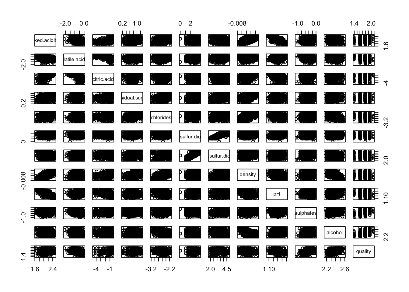
To get an insight of the outliers position we can use a scatter plot matrix.
pairs(redDat[, -grep("quality", colnames(redDat))])
We see that outliers seems to be on the higher and upper ends.
Now we look at the predictor values distribution:
oldpar = par(mfrow = c(6,2))
for ( i in 1:12 ) {
  truehist(redDat[[i]], xlab = names(redDat)[i], col = 'lightgreen', main = paste("Average =", signif(mean(redDat[[i]]),3)), nbins = 50)
}
par(oldpar)
We note that almost all distributions are positively skewed. Quality, pH and density are approximately normally distributed.
1.1.b: Outlier detection
For each variables, we consider observations that lie outside 1.5 * IQR as outliers.
redOutliers = c()
for ( i in 1:11 ) {
  stats = boxplot.stats(redDat[[i]])$stats
  bottom_outlier_rows = which(redDat[[i]] < stats[1])
  top_outlier_rows = which(redDat[[i]] > stats[5])
  redOutliers = c(redOutliers , top_outlier_rows[ !top_outlier_rows %in% redOutliers ] )
  redOutliers = c(redOutliers , bottom_outlier_rows[ !bottom_outlier_rows %in% redOutliers ] )
}
We use the Cook’s ditance to detect influential observations.
mod = lm(quality ~ ., data = redDat)
cooksd = cooks.distance(mod)
plot(cooksd, pch = "*", cex = 2, main = "Influential Obs by Cooks distance")
abline(h = 4*mean(cooksd, na.rm = T), col = "red")
head(redDat[cooksd > 4 * mean(cooksd, na.rm=T), ])
##    fixed.acidity volatile.acidity citric.acid residual.sugar chlorides
## 14           7.8            0.610        0.29            1.6     0.114
## 34           6.9            0.605        0.12           10.7     0.073
## 46           4.6            0.520        0.15            2.1     0.054
## 80           8.3            0.625        0.20            1.5     0.080
## 87           8.6            0.490        0.28            1.9     0.110
## 92           8.6            0.490        0.28            1.9     0.110
##    free.sulfur.dioxide total.sulfur.dioxide density   pH sulphates alcohol
## 14                   9                   29  0.9974 3.26      1.56     9.1
## 34                  40                   83  0.9993 3.45      0.52     9.4
## 46                   8                   65  0.9934 3.90      0.56    13.1
## 80                  27                  119  0.9972 3.16      1.12     9.1
## 87                  20                  136  0.9972 2.93      1.95     9.9
## 92                  20                  136  0.9972 2.93      1.95     9.9
##    quality
## 14       5
## 34       6
## 46       4
## 80       4
## 87       6
## 92       6
By looking at each row we can find out why it is influential:
- Row 14 and 46 have very low free.sulfur.dioxide.
- Row 34 have very high residual.sugar.
- Row 46 have very high alcohol.
- Row 87 and 92 have very high sulphates.
plot(lm(quality~citric.acid, data=redDat), which=c(5))
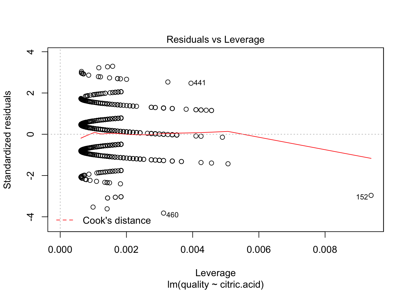
plot(lm(quality~total.sulfur.dioxide, data=redDat), which=c(5))
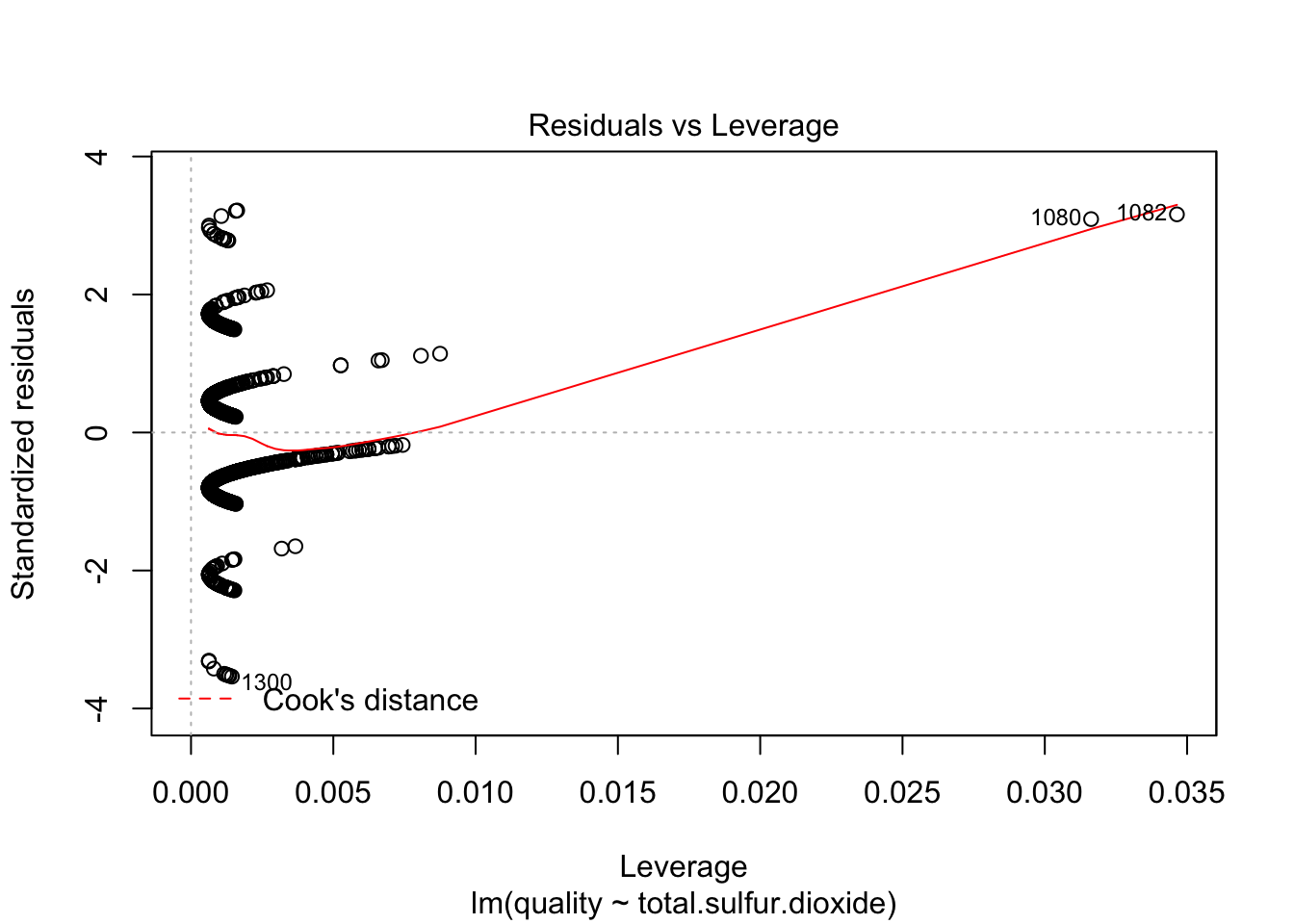
plot(lm(quality~sulphates, data=redDat), which=c(5))
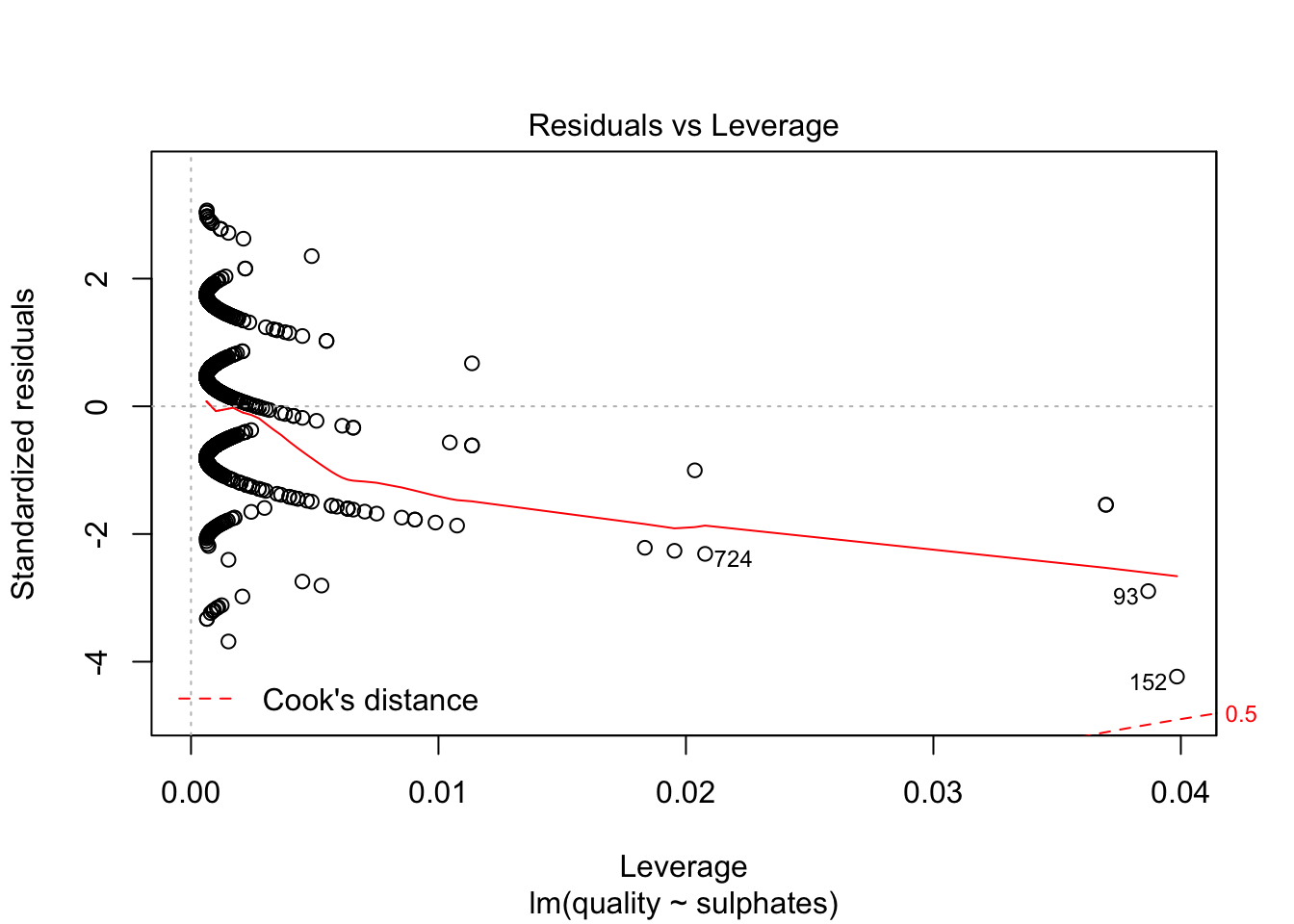
plot(lm(quality~alcohol, data=redDat), which=c(5))
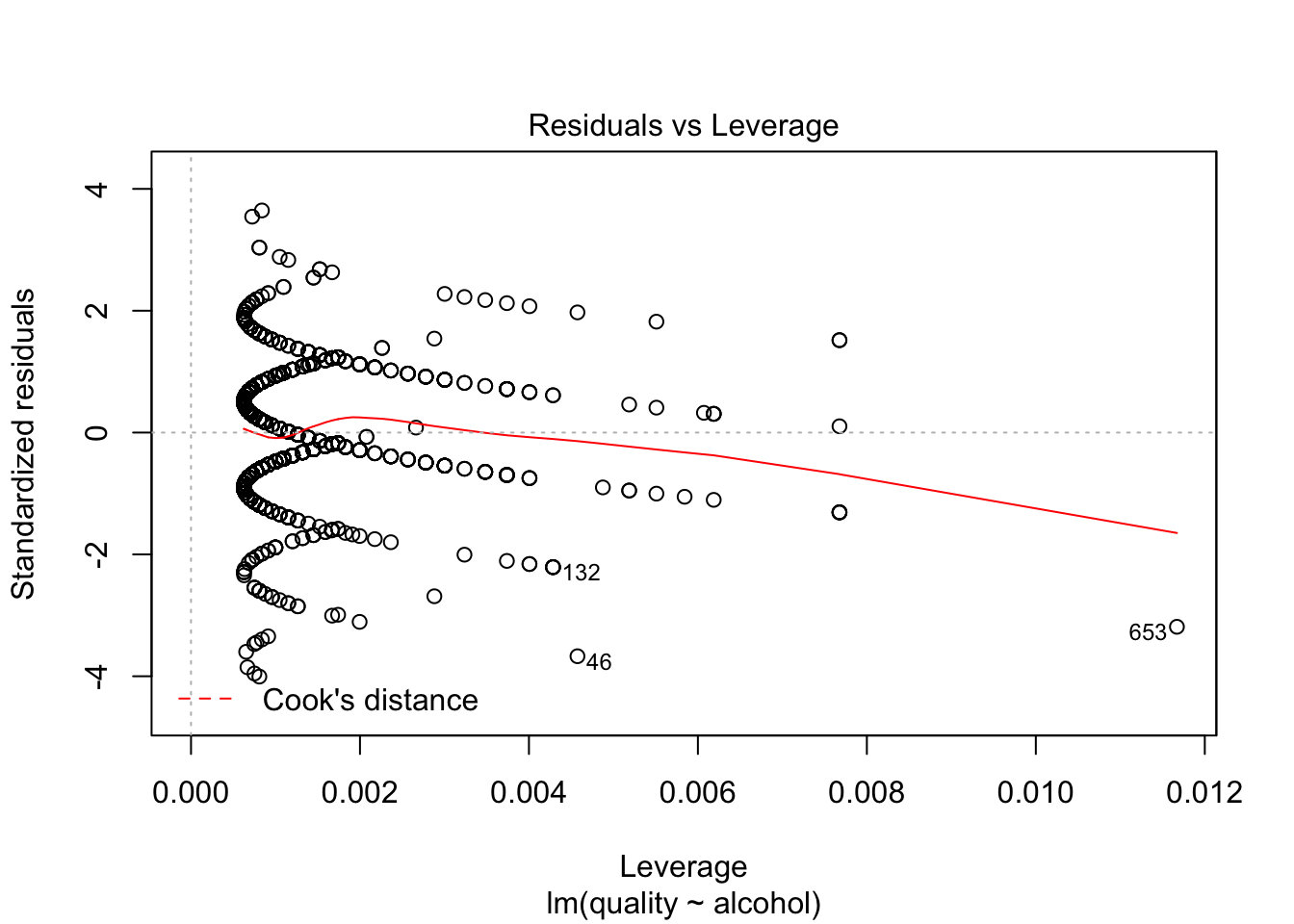
We remove all the ouliers in our list from the dataset and create new histograms:
coutliers = as.numeric(rownames(redDat[cooksd > 4 * mean(cooksd, na.rm=T), ]))
redOutliers = c(redOutliers , coutliers[ !coutliers %in% redOutliers ] )

cleanRedDat = redDat[-redOutliers, ]
oldpar = par(mfrow=c(6,2))

for ( i in 1:12 ) {
  truehist(cleanRedDat[[i]], xlab = names(cleanRedDat)[i], col = 'lightgreen', main = paste("Average =", signif(mean(cleanRedDat[[i]]),3)), nbins = 50)
}
par(oldpar)
By removing the outliers, the dataset size reduced to 1179 observations.
From the above plots, we can see that:
- fixed.acidity have a normal distribution.
- volatile.acidity seems to dispaly a bimodal normal distribution. Log-transforming it make the distribution becomes normal.
- citric.acid, free.sulfur.dioxide, total.sulfur.dioxide are skewed to the right.
- residual.sugar, chlorides, density, pH have a normal distribution.
- alcohol vary from 8.70 to 13.40. Most of the data are in the range 9-10.
Now, the variable distributions are approximatly normal except for residual.sugar which is unimodal and skewed to the right. This could be an interesting fact for further analysis.
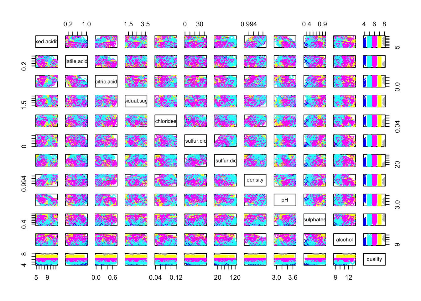
We now use a scatterplot matrice to roughly determine if there is a linear correlation between our variables:
pairs(cleanRedDat, col = cleanRedDat$quality, pch = cleanRedDat$quality)
pairs(cleanRedDat[,c(1, 8, 9, 10, 11)], col = cleanRedDat$quality, pch = cleanRedDat$quality)
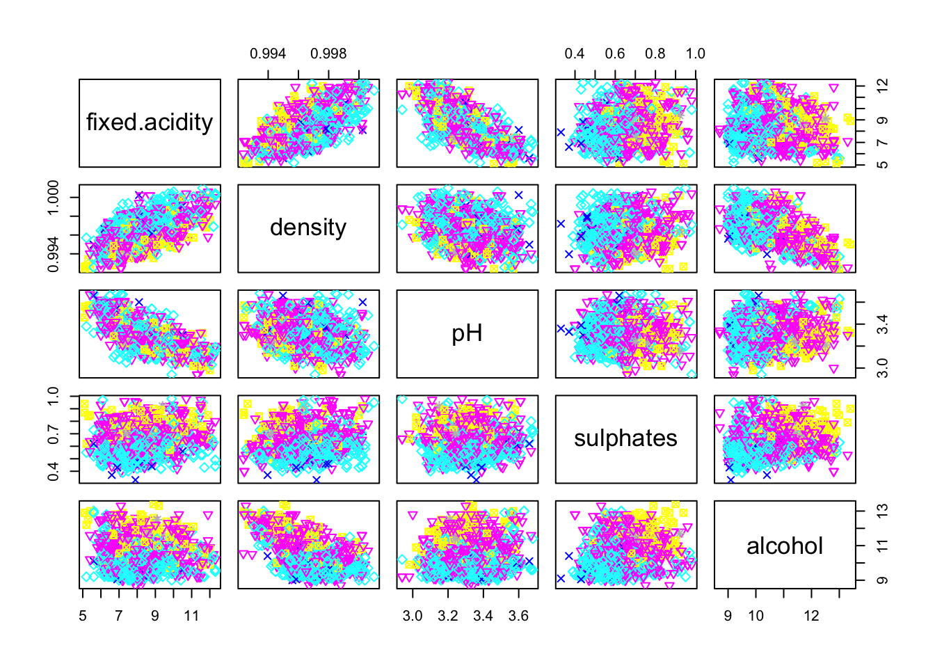
Only fixed.acidity/density and fixed.acidity/pH pairs seems to have a linear correlation.
We note a trend with the sulphates variable: the higher the sulphates value is, the better the quality. Idem for the alcohol variable.
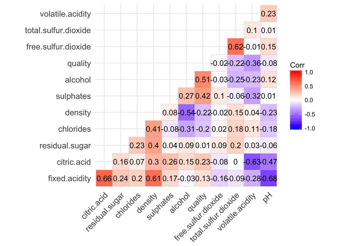
1.1.c: Correlation
The following correlation matrix confirm the strong correlation between fixed.acidity/density and fixed.acidity/pH. It also reveal the correlation between fixed.acidity/citric.acid, volatie.acidity/citric.acid and total.sulfur.dioxide/free.sulfur.dioxide.
The variables with the highest correlation with quality are alcohol and sulphates.
ggcorrplot(cor(cleanRedDat), hc.order = TRUE, type = "lower", lab = TRUE, insig = "blank")
colnames(sortByCorr(dataset = cleanRedDat, refColName = 'quality'))
##  [1] "quality"              "alcohol"              "sulphates"
##  [4] "volatile.acidity"     "citric.acid"          "total.sulfur.dioxide"
##  [7] "density"              "chlorides"            "fixed.acidity"
## [10] "pH"
1.3 Should we log-transform the data?
Log transformation is widely used to make data conform to normality and/or reduce variability of data. For the white wine, since our data are now close to the normal distribution, we don’t need to transform them.
In both case we can see in the following pairwise plots that log-transformation doesn’t improve linearity of the relationships between predictors and outcome.
pairs(log(cleanWhiteDat))
pairs(log(cleanRedDat))
1.4 Initial model performance
In order to have a point of comparison for the models to comes, we fit an initial model for each dataset with all variables:
whiteFit = lm(quality~., cleanWhiteDat)
redFit = lm(quality~., cleanRedDat)

summary(whiteFit)
##
## Call:
## lm(formula = quality ~ ., data = cleanWhiteDat)
##
## Residuals:
##      Min       1Q   Median       3Q      Max
## -2.92980 -0.51195 -0.04107  0.45599  2.45905
##
## Coefficients:
##                        Estimate Std. Error t value Pr(>|t|)
## (Intercept)           1.983e+02  2.702e+01   7.339 2.60e-13 ***
## fixed.acidity         1.521e-01  2.690e-02   5.652 1.69e-08 ***
## volatile.acidity     -1.887e+00  1.605e-01 -11.754  < 2e-16 ***
## citric.acid           6.282e-02  1.399e-01   0.449 0.653443
## residual.sugar        9.737e-02  1.011e-02   9.630  < 2e-16 ***
## chlorides            -3.589e+00  1.442e+00  -2.489 0.012865 *
## free.sulfur.dioxide   4.415e-03  1.038e-03   4.253 2.15e-05 ***
## total.sulfur.dioxide  2.656e-04  4.372e-04   0.607 0.543577
## density              -1.995e+02  2.738e+01  -7.287 3.81e-13 ***
## pH                    9.555e-01  1.275e-01   7.494 8.20e-14 ***
## sulphates             6.767e-01  1.243e-01   5.444 5.52e-08 ***
## alcohol               1.272e-01  3.375e-02   3.768 0.000167 ***
## ---
## Signif. codes:  0 '***' 0.001 '**' 0.01 '*' 0.05 '.' 0.1 ' ' 1
##
## Residual standard error: 0.7241 on 3987 degrees of freedom
## Multiple R-squared:  0.2623, Adjusted R-squared:  0.2602
## F-statistic: 128.9 on 11 and 3987 DF,  p-value: < 2.2e-16
# Calculate the MSE
mean(whiteFit$residuals^2)
## [1] 0.5226782summary(redFit)
##
## Call:
## lm(formula = quality ~ ., data = cleanRedDat)
##
## Residuals:
##      Min       1Q   Median       3Q      Max
## -1.92124 -0.36701 -0.05888  0.40757  1.87569
##
## Coefficients:
##                        Estimate Std. Error t value Pr(>|t|)
## (Intercept)           1.997e+01  2.672e+01   0.747  0.45513
## fixed.acidity         2.427e-02  3.024e-02   0.802  0.42246
## volatile.acidity     -8.010e-01  1.461e-01  -5.481 5.18e-08 ***
## citric.acid          -2.679e-01  1.657e-01  -1.617  0.10615
## residual.sugar        2.781e-03  4.985e-02   0.056  0.95552
## chlorides            -1.778e+00  1.341e+00  -1.327  0.18489
## free.sulfur.dioxide   3.327e-03  2.578e-03   1.290  0.19715
## total.sulfur.dioxide -2.882e-03  9.219e-04  -3.126  0.00181 **
## density              -1.602e+01  2.727e+01  -0.588  0.55687
## pH                   -5.468e-01  2.242e-01  -2.439  0.01489 *
## sulphates             1.657e+00  1.662e-01   9.973  < 2e-16 ***
## alcohol               2.810e-01  3.315e-02   8.478  < 2e-16 ***
## ---
## Signif. codes:  0 '***' 0.001 '**' 0.01 '*' 0.05 '.' 0.1 ' ' 1
##
## Residual standard error: 0.5752 on 1167 degrees of freedom
## Multiple R-squared:  0.3947, Adjusted R-squared:  0.389
## F-statistic: 69.17 on 11 and 1167 DF,  p-value: < 2.2e-16
# Calculate the MSE
mean(redFit$residuals^2)
## [1] 0.3274646White wine model:
- The most important variables are: fixed.acidity, volatile.acidity, residual.sugar, free.sulfur.dioxide, density, pH, sulphates and alcohol.
- citric.acid and total.sulfur.dioxide doesn’t seems to be relevant in this model.
- Adjusted R2 = 0.2602
- MSE = 0.5226782
Red wine model:
- The most important variables are: volatile.acidity, sulphates and alcohol.
- fixed.acidity, citric.acid, residual.sugar, chlorides, free.sulfur.dioxide and density doesn’t seems to be relevant in this model.
- Adjusted R2 = 0.389
- MSE = 0.3274646
2: Choose optimal models by exhaustive, forward and backward selection
2.1: White wine
Using the pre-processed white wine data, let’s use regsubsets to choose optimal set of variables for modeling wine quality using exhaustive, forward and backward methods:
testRegsubsets = function(dataset, yColName, methods, metrics) {
# Perform the given best subset selection methods and plot the given corresponding model
# metrics and the variable membership for each models
#
# Args:
# dataset: The data frame on which to perform subset selection methods
# yColName: The name of the outcome variable
# methods: Vector. The list of the subset selection methods to perform
# metrics: Vector. The list of metrics to plot
#
# Returns:
# Plot the given model metrics and the variable membership for each models
summaryMetrics = NULL
whichAll = list()
for (myMthd in methods) {
rsRes = regsubsets(dataset[, yColName]~ ., dataset[, -which(names(dataset) %in% yColName)], method = myMthd, nvmax = 11)
summRes = summary(rsRes)
whichAll[[myMthd]] = summRes$which
for (metricName in metrics) {
summaryMetrics = rbind(summaryMetrics,
data.frame(method = myMthd, metric = metricName,
nvars = 1:length(summRes[[metricName]]),
value = summRes[[metricName]]))
}
}
# Plot variable membership for each models
old.par = par(mfrow = c(1,2), ps = 16, mar = c(5,7,2,1))
for (myMthd in names(whichAll)) {
image(1:nrow(whichAll[[myMthd]]),
1:ncol(whichAll[[myMthd]]),
whichAll[[myMthd]], xlab = 'N(vars)', ylab = '',
xaxt = 'n', yaxt = 'n', breaks = c(-0.5, 0.5, 1.5),
col = c('white', 'lightblue1'), main = myMthd)
axis(1, 1:nrow(whichAll[[myMthd]]), rownames(whichAll[[myMthd]]))
axis(2, 1:ncol(whichAll[[myMthd]]), colnames(whichAll[[myMthd]]), las = 2)
}
par(old.par)
# Plot the model metrics
ggplot(summaryMetrics, aes(x = nvars, y = value, shape = method, colour = method)) + geom_path() + geom_point() + facet_wrap(~metric, scales = "free") + theme(legend.position = "top")
}
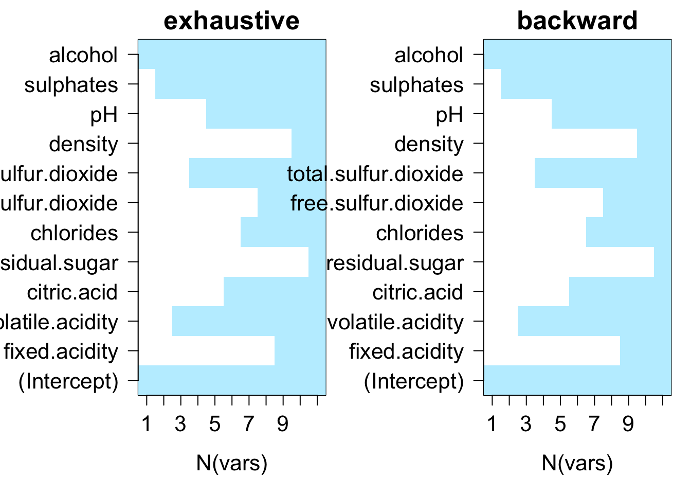
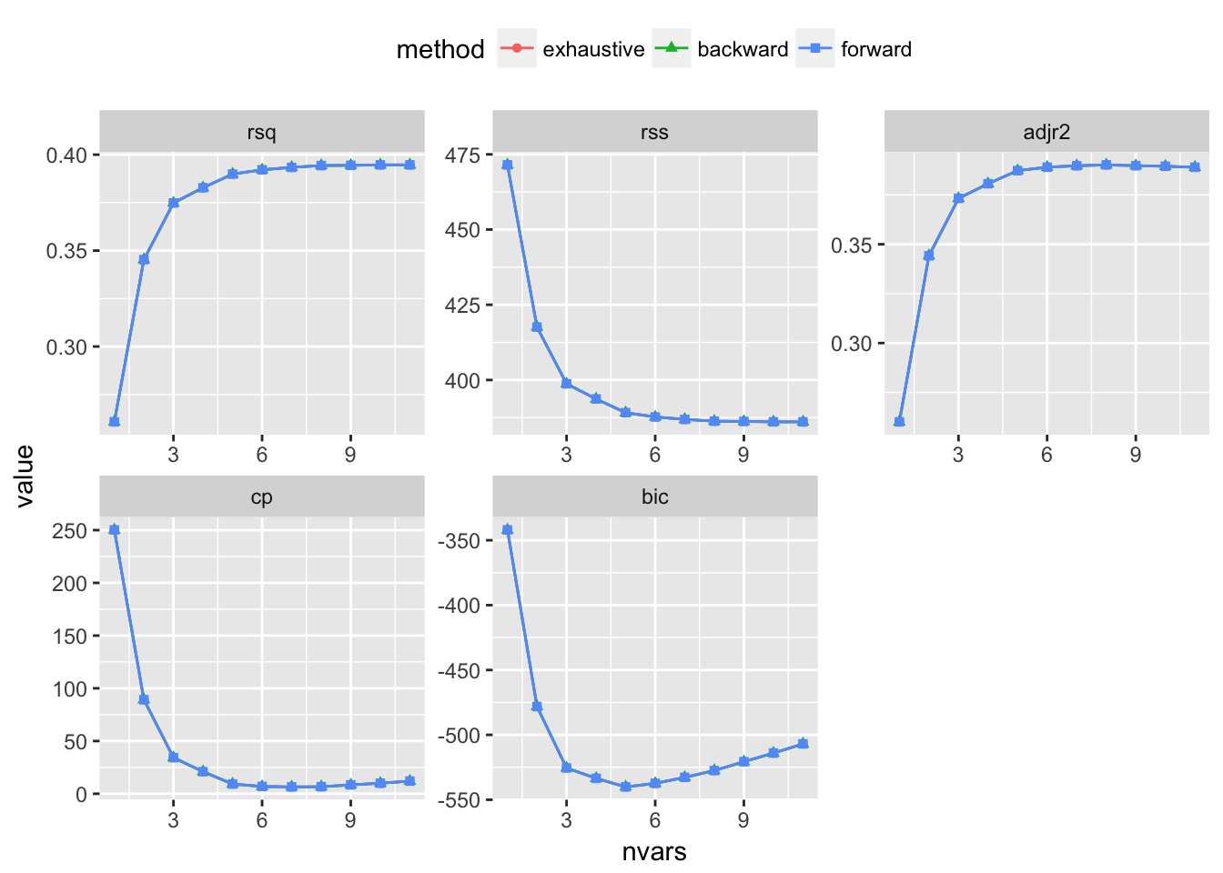
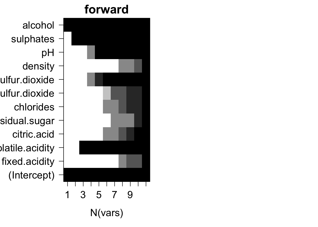
testRegsubsets(dataset = cleanWhiteDat, yColName = "quality", methods = c("exhaustive", "backward", "forward"), metrics = c("rsq", "rss", "adjr2", "cp", "bic"))
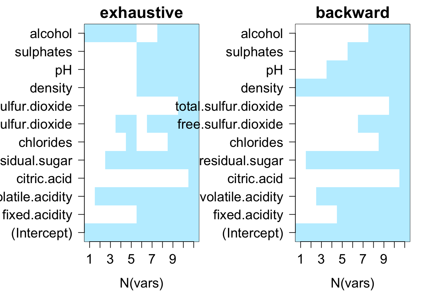
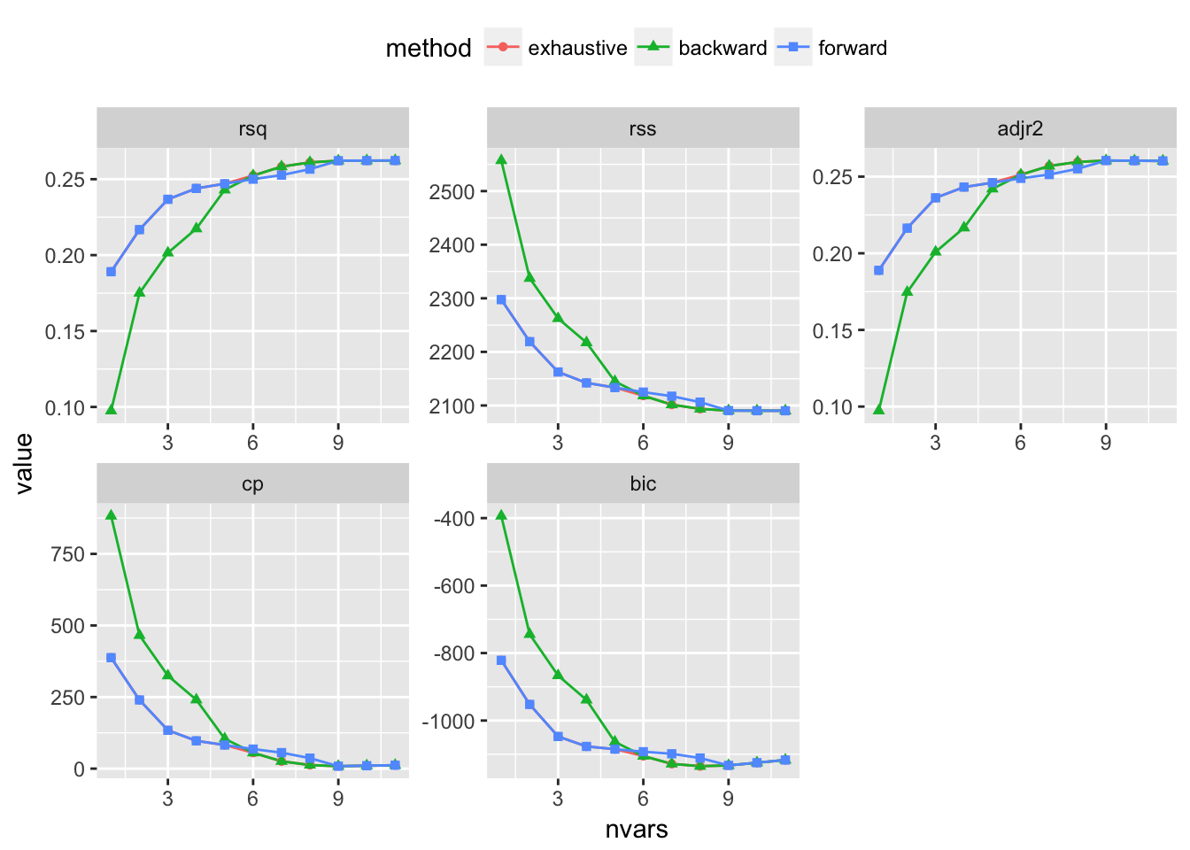
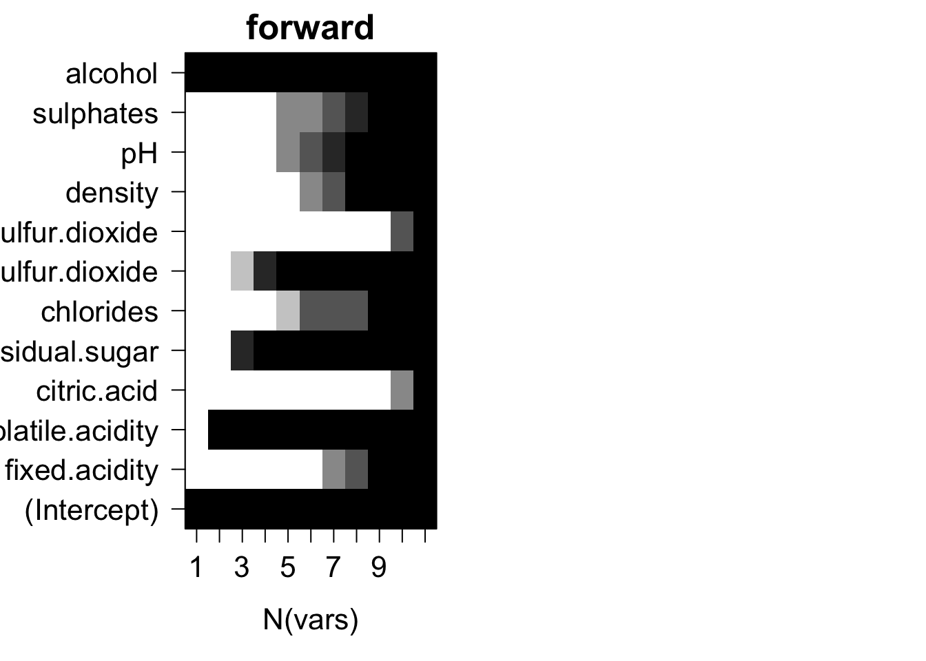
We see that exhaustive and forward subset selection methods came with models of very comparable performance by every associated metric while backward subset selection method have dissimilar performance when the number of predictor is less than 6, then performances are very comparable.
For all methods, increase in variable number appears to result in progressive improvement of the fit. It appear that the optimal model contain 9 variables. For all methods, the 9 variables model contain density, residual.sugar, volatile.acidity, pH, fixed.acidity, sulphates, free.sulfur.dioxide, alcohol and chlorides.
2.2: Red wine
testRegsubsets(dataset = cleanRedDat, yColName = "quality", methods = c("exhaustive", "backward", "forward"), metrics = c("rsq", "rss", "adjr2", "cp", "bic"))
We see that all subset selection methods came with models of very comparable performance by every associated metric. All except BIC reaches minimum when 6 out of 11 variables are in the model. Since the gain is very low between 5 and 6 for other metrics, it may be safe to said that the best model should contain 5 predictors.
For both backward and forward methods, the 5 variables model contain alcohol, sulphates, volatile.acidity, total.sulfur.dioxide and pH.
2.3 Comparison between red and white wine optimal models
Best models for both red wine and white wine contains alcohol, sulphates, volatile.acidity and pH.
The best model for red wine is the only one to contain total.sulfur.dioxide while the best model for white wine is the only one to contain density, residual.sugar, fixed.acidity, free.sulfur.dioxide and chlorides.
We now fit the best models found in this section for both dataset:
whiteFit2 = lm(quality~density + residual.sugar + volatile.acidity + pH + fixed.acidity + sulphates + free.sulfur.dioxide + alcohol + chlorides, cleanWhiteDat)
summary(whiteFit2)
##
## Call:
## lm(formula = quality ~ density + residual.sugar + volatile.acidity +
##     pH + fixed.acidity + sulphates + free.sulfur.dioxide + alcohol +
##     chlorides, data = cleanWhiteDat)
##
## Residuals:
##      Min       1Q   Median       3Q      Max
## -2.92869 -0.51616 -0.04218  0.46081  2.45222
##
## Coefficients:
##                       Estimate Std. Error t value Pr(>|t|)
## (Intercept)          1.928e+02  2.594e+01   7.430 1.32e-13 ***
## density             -1.939e+02  2.629e+01  -7.375 1.98e-13 ***
## residual.sugar       9.557e-02  9.810e-03   9.741  < 2e-16 ***
## volatile.acidity    -1.872e+00  1.546e-01 -12.110  < 2e-16 ***
## pH                   9.430e-01  1.265e-01   7.457 1.08e-13 ***
## fixed.acidity        1.509e-01  2.661e-02   5.670 1.53e-08 ***
## sulphates            6.809e-01  1.241e-01   5.485 4.39e-08 ***
## free.sulfur.dioxide  4.831e-03  8.271e-04   5.840 5.63e-09 ***
## alcohol              1.318e-01  3.320e-02   3.971 7.27e-05 ***
## chlorides           -3.505e+00  1.435e+00  -2.442   0.0147 *
## ---
## Signif. codes:  0 '***' 0.001 '**' 0.01 '*' 0.05 '.' 0.1 ' ' 1
##
## Residual standard error: 0.7239 on 3989 degrees of freedom
## Multiple R-squared:  0.2622, Adjusted R-squared:  0.2605
## F-statistic: 157.5 on 9 and 3989 DF,  p-value: < 2.2e-16
# Calculate the MSE
mean(whiteFit2$residuals^2)
## [1] 0.5227566redFit2 = lm(quality~alcohol + sulphates + volatile.acidity + total.sulfur.dioxide + pH, cleanRedDat)
summary(redFit2)
##
## Call:
## lm(formula = quality ~ alcohol + sulphates + volatile.acidity +
##     total.sulfur.dioxide + pH, data = cleanRedDat)
##
## Residuals:
##      Min       1Q   Median       3Q      Max
## -1.99787 -0.35463 -0.07231  0.42725  1.85975
##
## Coefficients:
##                       Estimate Std. Error t value Pr(>|t|)
## (Intercept)           3.608455   0.450967   8.002 2.93e-15 ***
## alcohol               0.300591   0.019112  15.728  < 2e-16 ***
## sulphates             1.634988   0.156711  10.433  < 2e-16 ***
## volatile.acidity     -0.693162   0.113788  -6.092 1.51e-09 ***
## total.sulfur.dioxide -0.002519   0.000666  -3.783 0.000163 ***
## pH                   -0.493500   0.133387  -3.700 0.000226 ***
## ---
## Signif. codes:  0 '***' 0.001 '**' 0.01 '*' 0.05 '.' 0.1 ' ' 1
##
## Residual standard error: 0.576 on 1173 degrees of freedom
## Multiple R-squared:  0.3899, Adjusted R-squared:  0.3873
## F-statistic: 149.9 on 5 and 1173 DF,  p-value: < 2.2e-16
# Calculate the MSE
mean(redFit2$residuals^2)
## [1] 0.3300581White wine model:
- All the variables in the model are important predictors.
- chlorides is the less relevant explainatory variable.
- Adjusted R2 = 0.2605 (0.389 in the previous model)
- MSE = 0.5227566 (doesn’t improve)
Red wine model:
- All the variables in the model are important predictors.
- Adjusted R2 = 0.3873 (0.389 in the previous model)
- MSE = 0.3300581 (doesn’t improve)
Compared to our initial models, performance doesn’t improve but the model is simpler because it contains less variables.
Optimal model by cross-validation
For each dataset, we will use the bootstrap resampling method to estimate test error for models with different numbers of variables and then compare with the results of the cross-validation method.
predict.regsubsets = function (object, newdata, id, ...){
  form = as.formula(object$call [[2]])
  mat = model.matrix(form ,newdata)
  coefi = coef(object, id = id)
  xvars = names(coefi)
  mat[, xvars]%*% coefi
}

# Best subset and bootstrap
resampleMSEregsubsetsWineDat = function(dataset, inpMthd, subsetMthd, nTries = 100) {
  if (!inpMthd %in% c("traintest", "bootstrap")) {
    stop("Unexpected resampling method!")
  }
  dfTmp = NULL
  whichSum = array(0, dim = c(ncol(dataset)-1, ncol(dataset), length(subsetMthd)), dimnames = list(NULL, colnames(model.matrix(quality~ ., dataset)), subsetMthd))
  for (iTry in 1:nTries) {
    trainIdx = NULL
    if (inpMthd == "traintest") {
      trainIdx = sample(nrow(dataset), nrow(dataset)/2)
    } else if (inpMthd == "bootstrap") {
      trainIdx = sample(nrow(dataset), nrow(dataset), replace = TRUE)
    }
    for (jSelect in subsetMthd) {
      rsTrain = regsubsets(quality~ ., dataset[trainIdx, ], nvmax = ncol(dataset)-1, method = jSelect)
      whichSum[,,jSelect] = whichSum[,,jSelect] + summary(rsTrain)$which
      for (kVarSet in 1:(ncol(dataset)-1)) {
        kCoef = coef(rsTrain, id = kVarSet)
        testPred = model.matrix(quality~ ., dataset[-trainIdx, ])[, names(kCoef)] %*% kCoef
        mseTest = mean((testPred-dataset[-trainIdx, "quality"])^2)
        dfTmp = rbind(dfTmp, data.frame(sim = iTry, sel = jSelect, vars = kVarSet, mse = c(mseTest, summary(rsTrain)$rss[kVarSet]/length(trainIdx)), trainTest = c("test", "train")))
      }
    }
  }
  list(mseAll = dfTmp, whichSum = whichSum, nTries = nTries)
}

# Cross-validation training and test error
xvalMSEregsubsetsWinedat = function(dataset, subsetMthd, nTries = 30, kXval = 5) {
  retRes = NULL
  for (iTry in 1:nTries) {
    xvalFolds = sample(rep(1:kXval, length.out = nrow(dataset)))
    # Try each method available in regsubsets
    # to select the best model of each size:
    for (jSelect in subsetMthd) {
      mthdTestErr2 = NULL
      mthdTrainErr2 = NULL
      mthdTestFoldErr2 = NULL
      for (kFold in 1:kXval) {
        rsTrain = regsubsets(quality~ ., dataset[xvalFolds != kFold, ], nvmax = 11, method = jSelect)
        # Calculate test error for each set of variables
        # using predict.regsubsets implemented above:
        nVarTestErr2 = NULL
        nVarTrainErr2 = NULL
        for (kVarSet in 1:11) {
          # make predictions for given number of variables and cross-validation fold:
          kCoef = coef(rsTrain, id = kVarSet)
          testPred = model.matrix(quality~ ., dataset[xvalFolds == kFold, ])[, names(kCoef)] %*% kCoef
          nVarTestErr2 = cbind(nVarTestErr2, (testPred-dataset[xvalFolds == kFold, "quality"])^2)
          trainPred = model.matrix(quality~ ., dataset[xvalFolds != kFold, ])[, names(kCoef)] %*% kCoef
          nVarTrainErr2 = cbind(nVarTrainErr2, (trainPred-dataset[xvalFolds != kFold, "quality"])^2)
        }
        # accumulate training and test errors over all cross-validation folds:
        mthdTestErr2 = rbind(mthdTestErr2, nVarTestErr2)
        mthdTestFoldErr2 = rbind(mthdTestFoldErr2, colMeans(nVarTestErr2))
        mthdTrainErr2 = rbind(mthdTrainErr2, nVarTrainErr2)
      }
      # add to data.frame for future plotting:
      retRes = rbind(retRes,
                    data.frame(sim = iTry, sel = jSelect, vars = 1:ncol(nVarTrainErr2), mse = colMeans(mthdTrainErr2), trainTest = "train"),
                    data.frame(sim = iTry, sel = jSelect, vars = 1:ncol(nVarTrainErr2), mse = colMeans(mthdTestErr2), trainTest = "test"))
    }
  }
  retRes
}
3.1: White wine
3.1.a: The bootstrap
Resample by splitting dataset into training and test:
whiteBootRes = resampleMSEregsubsetsWineDat(cleanWhiteDat, "bootstrap", c("exhaustive", "backward", "forward"), 30)
Plot resulting training and test MSE:
ggplot(whiteBootRes$mseAll, aes(x = factor(vars), y = mse, colour = sel)) + geom_boxplot()+facet_wrap(~trainTest)
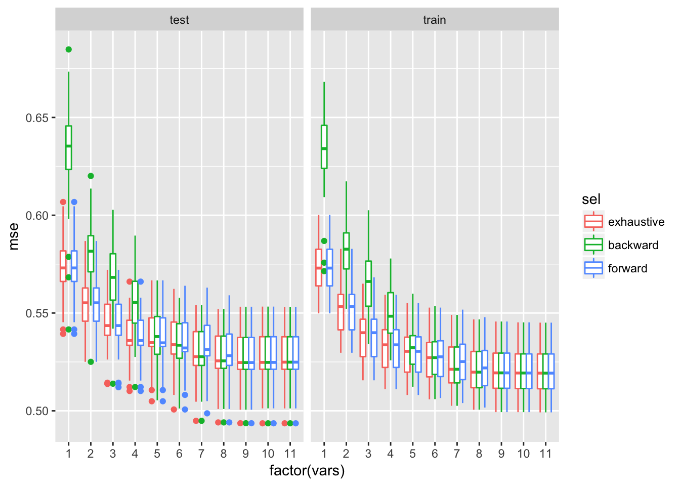
Test error improves by increasing model size up to about 9 variables. Median test MSE of the larger model is comparable to the lower quartile of MSE for the smaller model. Perhaps going from 8 to 9 variables also on average decreases test MSE as well, although that decrease is small comparing to the variability observed across resampling tries.
The test MSEs on models with 9 and 10 variables are very comparable but it is best to select the model with the least variables. This compromise between completeness and performance seems to justified to me since increasing the model complexity would just slightly improve it.
old.par = par(mfrow = c(1, 2), ps = 16, mar = c(5, 7, 2, 1))
for (myMthd in dimnames(whiteBootRes$whichSum)[[3]]) {
  tmpWhich = whiteBootRes$whichSum[,,myMthd] / whiteBootRes$nTries
  image(1:nrow(tmpWhich), 1:ncol(tmpWhich), tmpWhich,
        xlab = "N(vars)", ylab = "", xaxt = "n", yaxt = "n", main = myMthd,
        breaks = c(-0.1, 0.1, 0.25, 0.5, 0.75, 0.9, 1.1),
        col = gray(seq(1, 0, length = 6)))
  axis(1, 1:nrow(tmpWhich), rownames(tmpWhich))
  axis(2, 1:ncol(tmpWhich), colnames(tmpWhich), las = 2)
}
par(old.par)
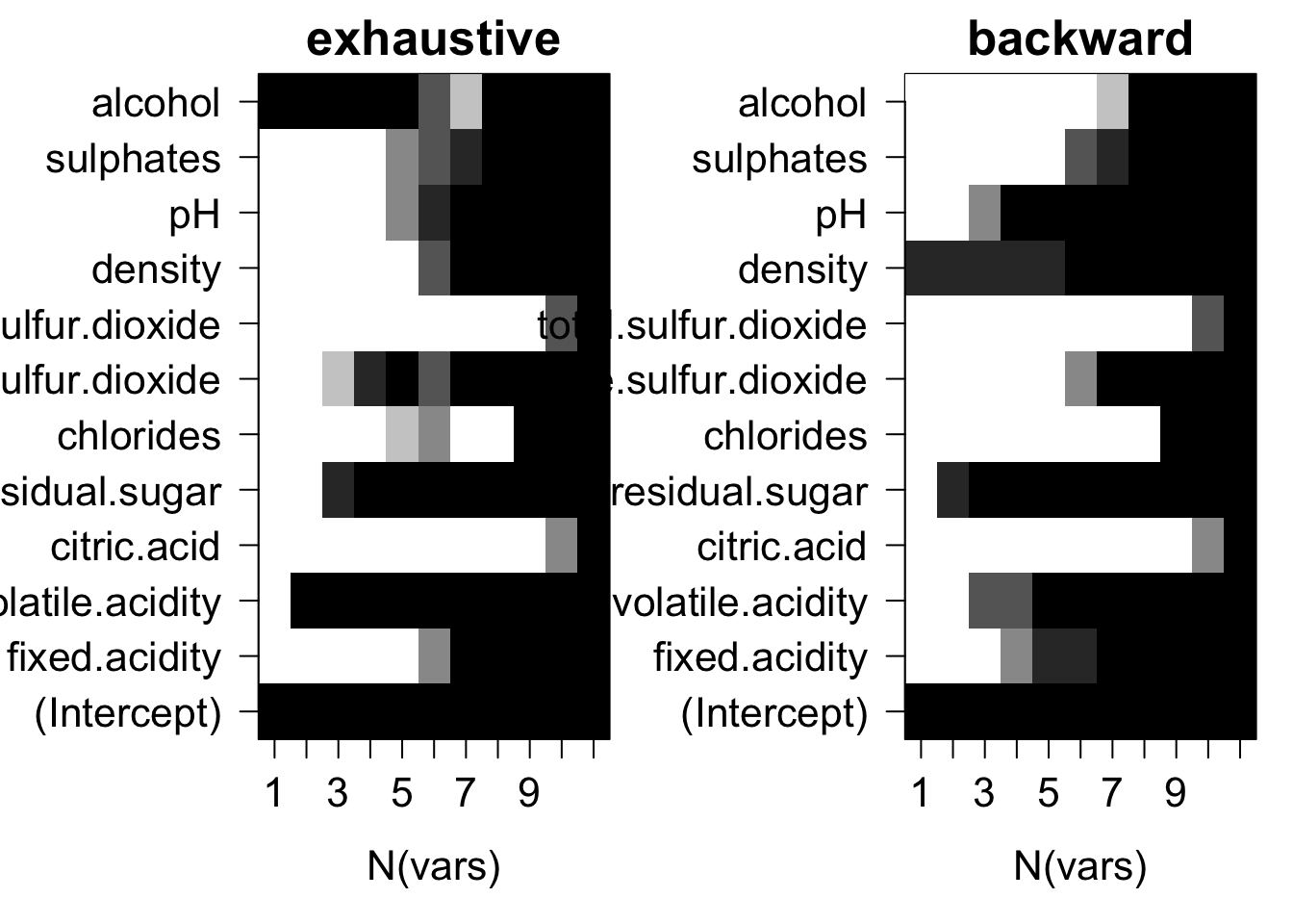
Plots of average variable membership in the model suggest that:
- citric.acid and total.sulfur.dioxide doesn’t get included until all variables are required to be in the model.
- either alcohol or density or CACH are included when only one variable is chosen.
- for models with nine variables chlorides or fixed.acidity is the last variable in the model.
3.1.b: K-fold Cross-validation
We can compare the bootstrap estimate test error with the results of the cross-validation resampling method on the same dataset:
dfTmp = rbind(data.frame(xvalMSEregsubsetsWinedat(cleanWhiteDat, c("exhaustive", "backward", "forward"), 30, kXval = 2), xval = "2-fold"),
data.frame(xvalMSEregsubsetsWinedat(cleanWhiteDat, c("exhaustive", "backward", "forward"), 30, kXval = 5), xval = "5-fold"),
data.frame(xvalMSEregsubsetsWinedat(cleanWhiteDat, c("exhaustive", "backward", "forward"), 30, kXval = 10), xval = "10-fold"))
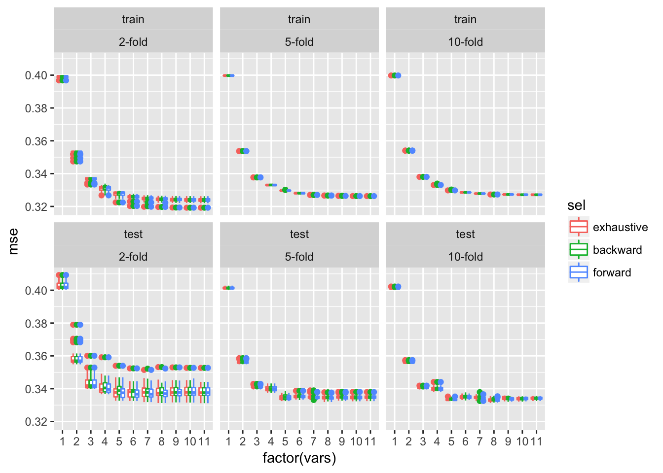
ggplot(dfTmp, aes(x = factor(vars), y = mse, colour = sel)) + geom_boxplot()+facet_wrap(~trainTest+xval)
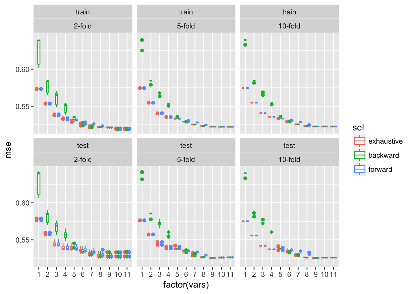
The average test error estimates obtained by cross-validation are approximately comparable to those obtained by bootstrap approaches and are by far less variable across multiple rounds of cross-validation, in particular for higher numbers of cross-validation folds.
In conclusion the best model here contains 9 variables: alcohol, sulphates, pH, density, free.sulfur.dioxide, chlorides, residual.suger, volatile.acidity and fixed.acidity.
3.2: Red wine
3.2.a: The bootstrap
As for the white wine data we resample using the bootstrap method and plot resulting training and test MSE:
redBootRes = resampleMSEregsubsetsWineDat(cleanRedDat, "bootstrap", c("exhaustive", "backward", "forward"), 30)
ggplot(redBootRes$mseAll, aes(x = factor(vars), y = mse, colour = sel)) + geom_boxplot()+facet_wrap(~trainTest)
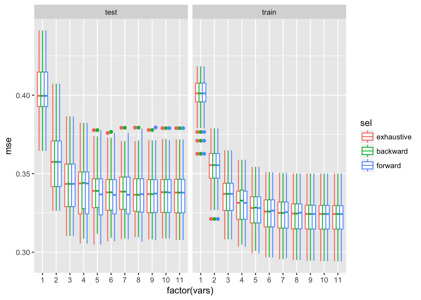
Test error improves by increasing model size up to about 5 variables. Median test MSE of the larger model is comparable to the lower quartile of MSE for the smaller model. Since test MSEs on models with more than 5 variables are very comparable the 5 variables model is considered as the best.
old.par = par(mfrow = c(1, 2), ps = 16, mar = c(5, 7, 2, 1))
for (myMthd in dimnames(redBootRes$whichSum)[[3]]) {
  tmpWhich = redBootRes$whichSum[,,myMthd] / redBootRes$nTries
  image(1:nrow(tmpWhich), 1:ncol(tmpWhich), tmpWhich,
        xlab = "N(vars)", ylab = "", xaxt = "n", yaxt = "n", main = myMthd,
        breaks = c(-0.1, 0.1, 0.25, 0.5, 0.75, 0.9, 1.1),
        col = gray(seq(1, 0, length = 6)))
  axis(1, 1:nrow(tmpWhich), rownames(tmpWhich))
  axis(2, 1:ncol(tmpWhich), colnames(tmpWhich), las = 2)
}
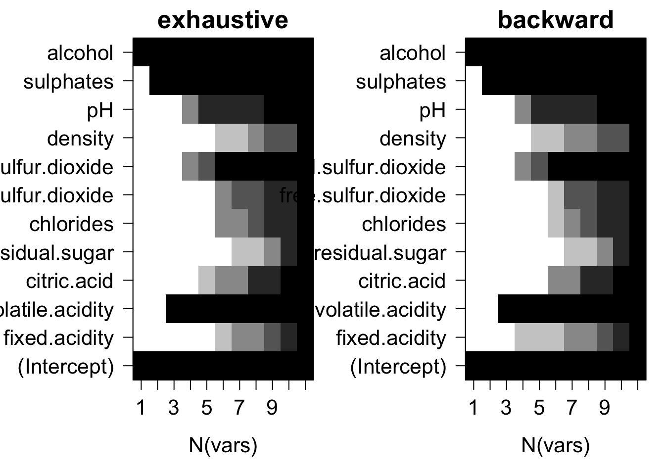
Plots of average variable membership in the model suggest that:
- residual.sugar or density doesn’t get included until all variables are required to be in the model.
- alcohol is included when only one variable is chosen.
- for models with five variables ph or total.sulfur.dioxide is the last variable in the model.
3.2.b: K-fold Cross-validation
As previously we can compare the bootstrap estimate test error with the results of the cross-validation resampling method on the same dataset:
dfTmp = rbind(data.frame(xvalMSEregsubsetsWinedat(cleanRedDat, c("exhaustive", "backward", "forward"), 30, kXval = 2), xval = "2-fold"),
               data.frame(xvalMSEregsubsetsWinedat(cleanRedDat, c("exhaustive", "backward", "forward"), 30, kXval = 5), xval = "5-fold"),
               data.frame(xvalMSEregsubsetsWinedat(cleanRedDat, c("exhaustive", "backward", "forward"), 30, kXval = 10), xval = "10-fold"))
ggplot(dfTmp, aes(x = factor(vars), y = mse, colour = sel)) + geom_boxplot()+facet_wrap(~trainTest+xval)
The same conclusion as for the white wine dataset holds here: The average test error estimates obtained by cross-validation are approximately comparable to those obtained by bootstrap approaches and are by far less variable across multiple rounds of cross-validation, in particular for higher numbers of cross-validation folds.
In conclusion the best model here contains 5 variables: alcohol, suplhates, pH, total.sulfur.dioxide, volatile.acidity.
3.3: Comparing red and white wine models
The best model for red wine contains only 5 variables while the best model for white wine contains 9. It seems to less complex to explain and predict red wine quality.
This results are similar to what we found using regsubsets in the previous task.
The resulting white model is the same as the one we found in sub-problem 2. It contains the 9 following variables: alcohol, sulphates, pH, density, free.sulfur.dioxide, chlorides, residual.sugar, volatile.acidity and fixed.acidity.
As for the white wine model, the best red wine model here is the same as previously. It contains the following 5 variables: alcohol, suplhates, pH, total.sulfur.dioxide (or free.sulfur.dioxide) and volatile.acidity.
Both contain alcohol, suplhates, pH and volatile.acidity, which may indicate that this variables are the most important predictors for quality, whatever the wine color.
4: lasso/ridge
Use regularized approaches (i.e. lasso and ridge) to model quality of red and white wine (separately). Compare resulting models (in terms of number of variables and their effects) to those selected in the previous two tasks (by regsubsets and resampling), comment on differences and similarities among them.
4.1: White wine
4.1.a: Lasso regression
# x = model.matrix(quality~ ., cleanWhiteDat[, -8])[, -1]
x = model.matrix(quality~ ., cleanWhiteDat)[, -1]
y = cleanWhiteDat[, "quality"]
lassoRes = glmnet(x, y, alpha = 1)
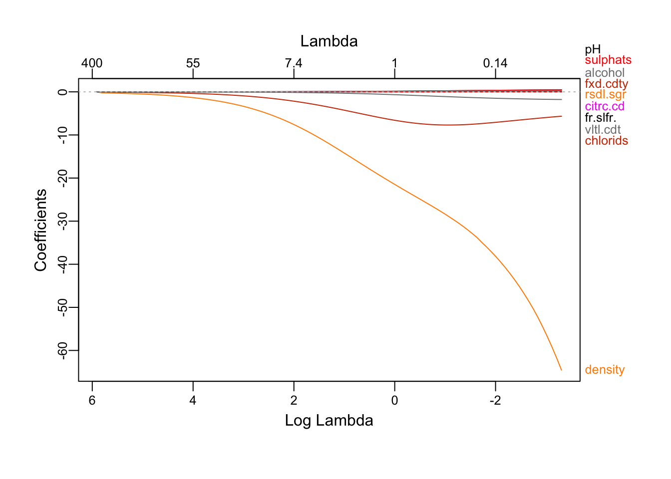
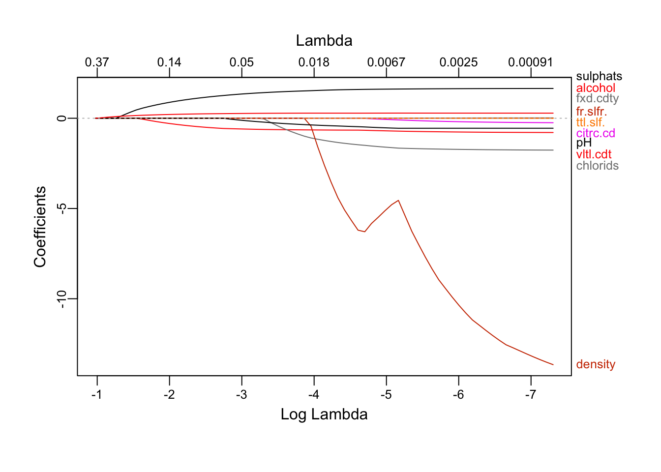
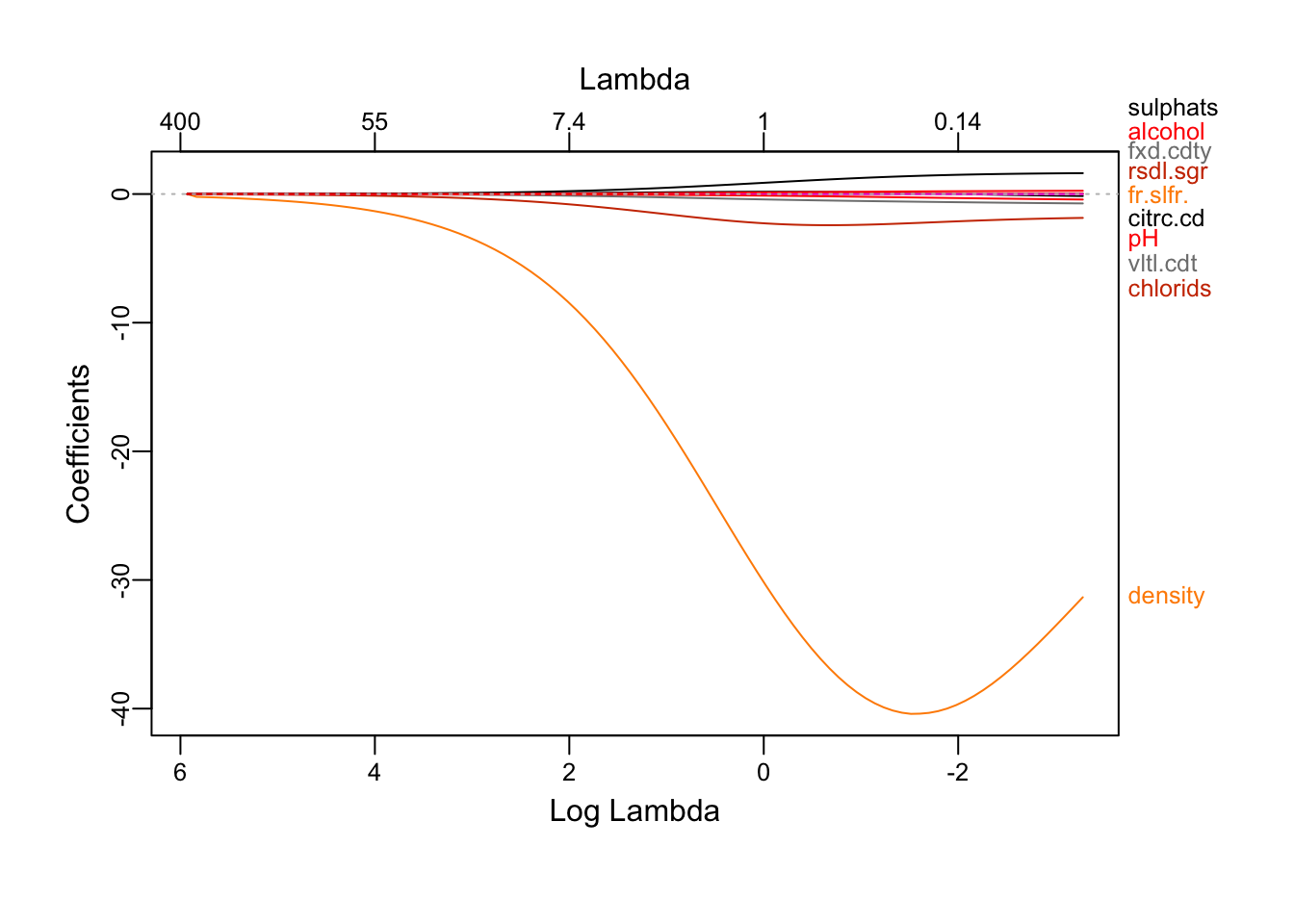
plot_glmnet(lassoRes)
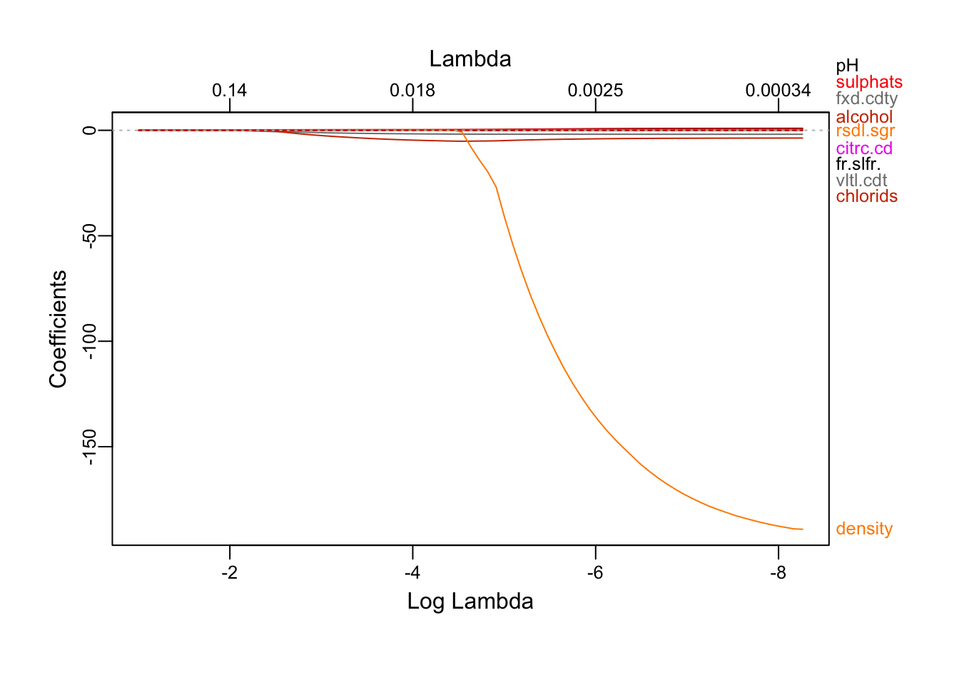
We see that as the constraint is relaxed, more attributes shows up. alcohol is first to emmerge, followed by volatile.acidity and chlorides and then pH, residual.sugar, sulphates… and finally, density. Because the lasso can be view as a attributes selection method, the attributes emerging first are the one who explains the most of the outcome. We also note that all the coefficients are positive except density, chlorids and volatile.acidity.
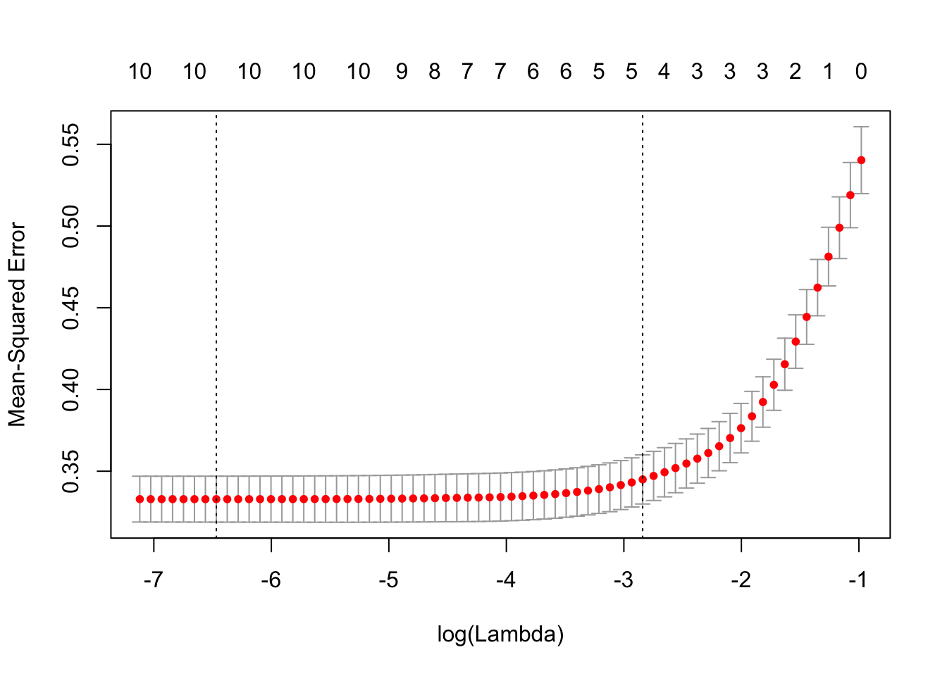
cvLassoRes = cv.glmnet(x, y, alpha = 1)
plot(cvLassoRes)
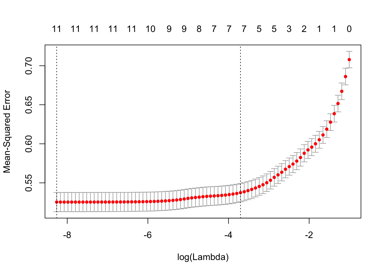
cvLassoRes = cv.glmnet(x, y, alpha = 1, lambda = 10^((-200:20)/80))
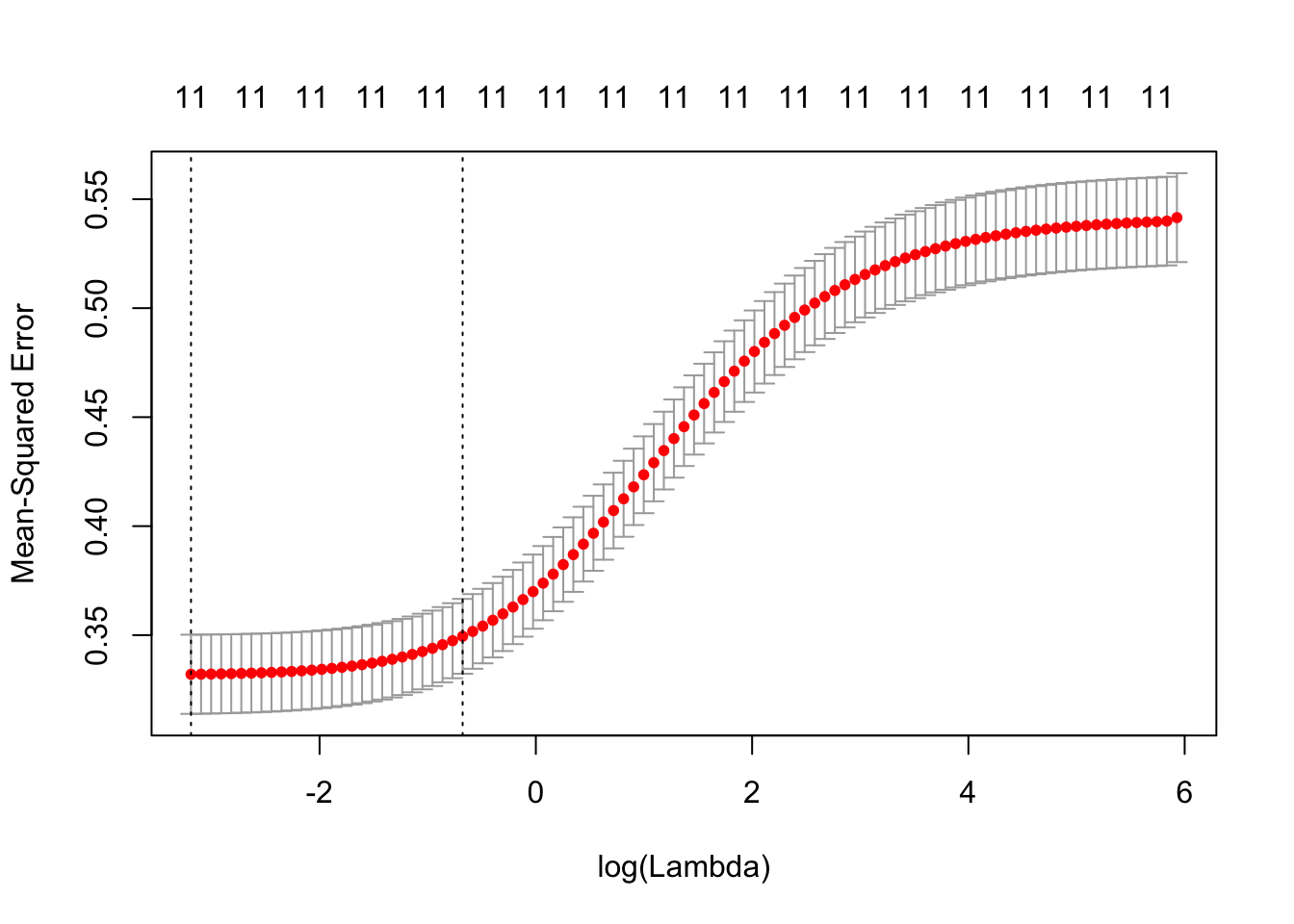
plot(cvLassoRes)
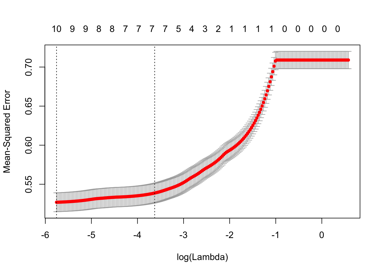
This plot of cv.glmnet shows us that as the model complexity decrease, the MSE increase. However, as there is at least 7 attributes in the model, the MSE stay low.
predict(lassoRes, type = "coefficients", s = cvLassoRes$lambda.min)
## 12 x 1 sparse Matrix of class "dgCMatrix"
##                                  1
## (Intercept)           1.206083e+02
## fixed.acidity         8.571880e-02
## volatile.acidity     -1.864622e+00
## citric.acid           1.077039e-02
## residual.sugar        6.781266e-02
## chlorides            -4.164688e+00
## free.sulfur.dioxide   4.679359e-03
## total.sulfur.dioxide  .
## density              -1.205164e+02
## pH                    6.610149e-01
## sulphates             5.397290e-01
## alcohol               2.115829e-01
Optimal (in min sens) model by lasso includes all variables except total.sulfur.dioxide.
predict(lassoRes, type = "coefficients", s = cvLassoRes$lambda.1se)
## 12 x 1 sparse Matrix of class "dgCMatrix"
##                                 1
## (Intercept)           2.666865609
## fixed.acidity         .
## volatile.acidity     -1.526877996
## citric.acid           .
## residual.sugar        0.013638167
## chlorides            -4.054700600
## free.sulfur.dioxide   0.003589056
## total.sulfur.dioxide  .
## density               .
## pH                    0.095449835
## sulphates             0.098144930
## alcohol               0.311437899
Unlike what was seen above, optimal (in min-1SE sense) model by lasso includes 7 variables: volatile.acidity, residual.sugar, chlorides, free.sulfur.dioxide, pH, sulphates, alcohol. fixed.acidity, citric.acid, total.sulfur.dioxide and density are left out.
For a better understanding of these results we use resampling to estimate test error of lasso models fit to training data and stability of the variable selection by lasso across different splits of data into training and test.
dfTmp = NULL
# Get the coefficients index after a lasso regression
coefs = predict(lassoRes, type = "coefficients", s = cvLassoRes$lambda.1se)
coefsIdx = which(coefs != 0)
lassoLnWhiteDat = cleanWhiteDat[, coefsIdx]
whichSum = array(0,dim = c((length(coefsIdx)-1), length(coefsIdx), 3),
dimnames = list(NULL, colnames(model.matrix(quality~ ., lassoLnWhiteDat)),
c("exhaustive", "backward", "forward")))
# Split data into training and test 30 times:
nTries <- 30
for ( iTry in 1:nTries ) {
bTrain = sample(rep(c(TRUE, FALSE), length.out = nrow(lassoLnWhiteDat)))
# Try each method available in regsubsets
# to select the best model of each size:
for ( jSelect in c("exhaustive", "backward", "forward") ) {
rsTrain = regsubsets(quality~ ., lassoLnWhiteDat[bTrain,], nvmax = 11, method = jSelect)
# Add up variable selections:
whichSum[,,jSelect] = whichSum[,,jSelect] + summary(rsTrain)$which
# Calculate test error for each set of variables
# using predict.regsubsets implemented above:
for ( kVarSet in 1:(length(coefsIdx)-1) ) {
# make predictions:
testPred = predict(rsTrain, lassoLnWhiteDat[!bTrain,], id = kVarSet)
# calculate MSE:
mseTest = mean((testPred-lassoLnWhiteDat[!bTrain, "quality"])^2)
# add to data.frame for future plotting:
dfTmp = rbind(dfTmp, data.frame(sim = iTry, sel = jSelect, vars = kVarSet,
mse = c(mseTest, summary(rsTrain)$rss[kVarSet]/sum(bTrain)), trainTest = c("test","train")))
}
}
}
# plot MSEs by training/test, number of
# variables and selection method:
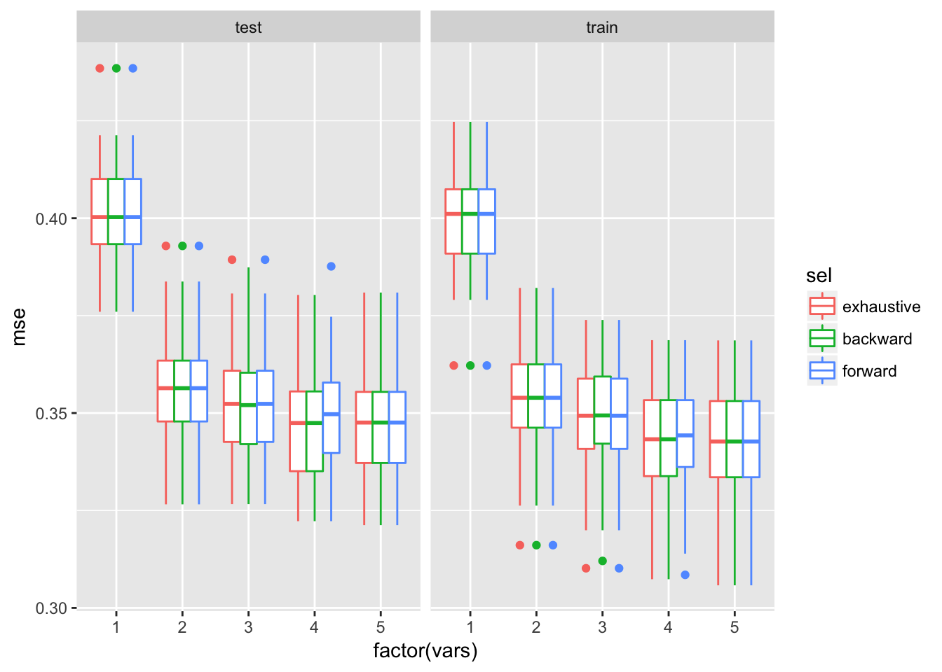
ggplot(dfTmp, aes(x = factor(vars), y = mse, colour = sel)) + geom_boxplot()+facet_wrap(~trainTest)
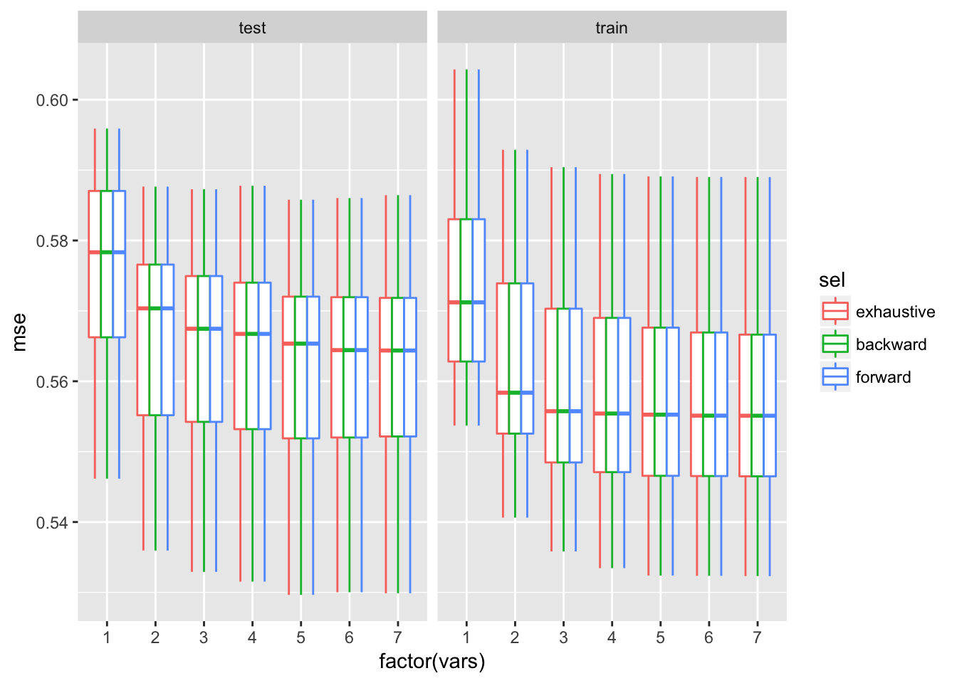
As we can see, the 5, 6 and 7 variables models are very similar.
whiteLassoCoefCnt = 0
whiteLassoMSE = NULL
for (iTry in 1:30) {
  bTrain = sample(rep(c(TRUE, FALSE), length.out = nrow(x)))
  cvLassoTrain = cv.glmnet(x[bTrain, ], y[bTrain], alpha = 1, lambda = 10^((-120:0)/20))
  lassoTrain = glmnet(x[bTrain, ], y[bTrain], alpha = 1, lambda = 10^((-120:0)/20))
  lassoTrainCoef = predict(lassoTrain, type = "coefficients", s = cvLassoTrain$lambda.1se)
  whiteLassoCoefCnt = whiteLassoCoefCnt + (lassoTrainCoef[-1, 1] != 0)
  lassoTestPred = predict(lassoTrain, newx = x[!bTrain, ], s = cvLassoTrain$lambda.1se)
  whiteLassoMSE = c(whiteLassoMSE, mean((lassoTestPred-y[!bTrain])^2))
}
mean(whiteLassoMSE)
## [1] 0.5464914quantile(whiteLassoMSE)
##        0%       25%       50%       75%      100%
## 0.5167767 0.5356218 0.5488897 0.5565241 0.5698861
whiteLassoCoefCnt
##        fixed.acidity     volatile.acidity          citric.acid
##                    1                   30                    1
##       residual.sugar            chlorides  free.sulfur.dioxide
##                   30                   29                   30
## total.sulfur.dioxide              density                   pH
##                    0                    0                   16
##            sulphates              alcohol
##                   15                   30
4.1.b: Ridge regression
ridgeRes = glmnet(x, y, alpha = 0)
plot_glmnet(ridgeRes)
We see that as the λ decrease, more attributes shows up.
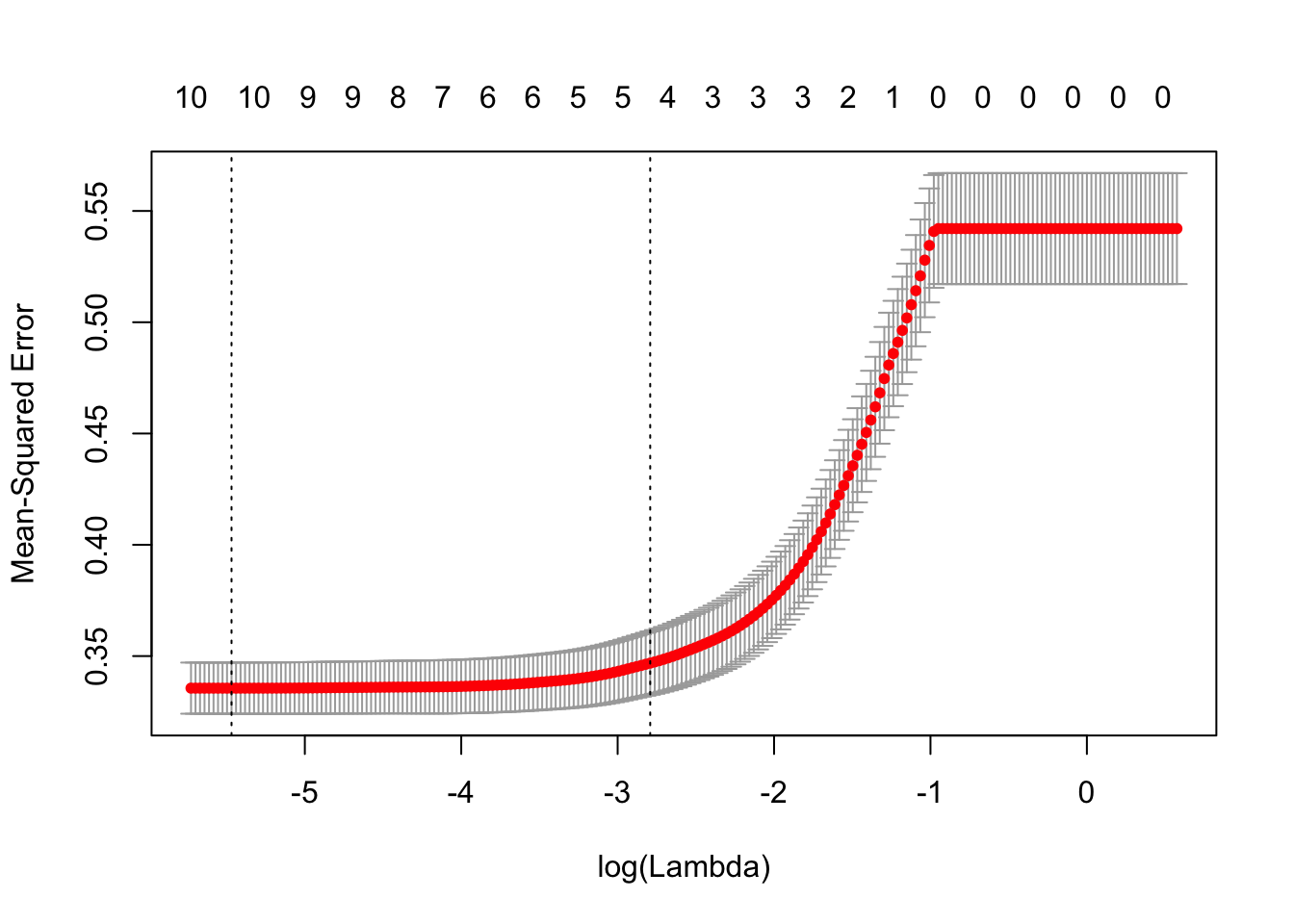
cvRidgeRes = cv.glmnet(x, y, alpha = 0)
plot(cvRidgeRes)
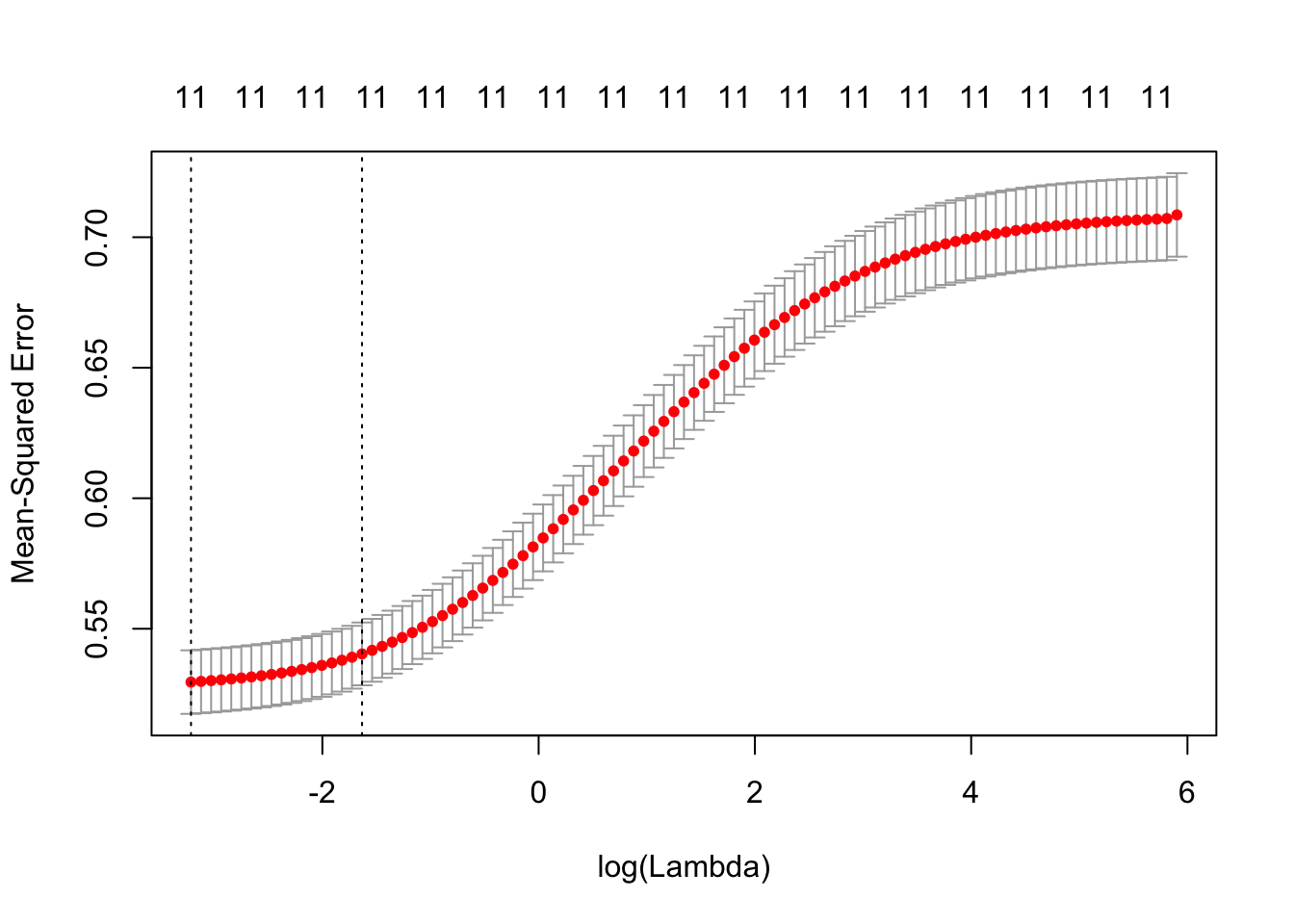
The cv.glmnet plot shows us that the 11 variable model has a low error as long as the lambda value is below -1.
cvRidgeRes$lambda.min
## [1] 0.04016908cvRidgeRes$lambda.1se
## [1] 0.1953263predict(ridgeRes, type = "coefficients", s = cvRidgeRes$lambda.min)
## 12 x 1 sparse Matrix of class "dgCMatrix"
##                                  1
## (Intercept)           6.298621e+01
## fixed.acidity         4.321403e-02
## volatile.acidity     -1.762595e+00
## citric.acid           3.957287e-02
## residual.sugar        4.333255e-02
## chlorides            -5.739301e+00
## free.sulfur.dioxide   5.289764e-03
## total.sulfur.dioxide -3.744853e-04
## density              -6.184207e+01
## pH                    4.729349e-01
## sulphates             4.547114e-01
## alcohol 2.545227e-01predict(ridgeRes, type = "coefficients", s = cvRidgeRes$lambda.1se)
## 12 x 1 sparse Matrix of class "dgCMatrix"
##                                  1
## (Intercept)           3.650802e+01
## fixed.acidity         1.204128e-02
## volatile.acidity     -1.358885e+00
## citric.acid           9.474516e-02
## residual.sugar        2.245641e-02
## chlorides            -7.436166e+00
## free.sulfur.dioxide   4.781170e-03
## total.sulfur.dioxide -6.107318e-04
## density              -3.381372e+01
## pH                    3.076046e-01
## sulphates             3.117719e-01
## alcohol               2.129788e-01
ridgeResScaled = glmnet(scale(x), y, alpha = 0)
cvRidgeResScaled = cv.glmnet(scale(x), y, alpha = 0, lambda = 10^((-50:60)/20))
predict(ridgeResScaled, type = "coefficients", s = cvRidgeResScaled$lambda.1se)
## 12 x 1 sparse Matrix of class "dgCMatrix"
##                                 1
## (Intercept)           5.950737684
## fixed.acidity         0.014457345
## volatile.acidity     -0.115066652
## citric.acid           0.006527448
## residual.sugar        0.139162023
## chlorides            -0.069276285
## free.sulfur.dioxide   0.076193500
## total.sulfur.dioxide -0.023026773
## density              -0.112759045
## pH                    0.048630857
## sulphates             0.035401235
## alcohol               0.283546517
The impact of alcohol and volatile.acidity is made more apparent.
whiteRidgeCoefCnt = 0
whiteRedridgeCoefAve = 0
whiteRidgeMSE = NULL
for ( iTry in 1:30 ) {
  bTrain = sample(rep(c(TRUE, FALSE), length.out = nrow(x)))
  cvridgeTrain = cv.glmnet(x[bTrain, ], y[bTrain], alpha = 0, lambda = 10^((-50:50)/20))
  ridgeTrain = glmnet(x[bTrain, ], y[bTrain], alpha = 0, lambda = 10^((-50:50)/20))
  ridgeTrainCoef = predict(ridgeTrain, type = "coefficients", s = cvridgeTrain$lambda.1se)
  whiteRidgeCoefCnt = whiteRidgeCoefCnt + (ridgeTrainCoef[-1,1] != 0)
  whiteRedridgeCoefAve = whiteRedridgeCoefAve + ridgeTrainCoef[-1, 1]
  ridgeTestPred = predict(ridgeTrain, newx = x[!bTrain, ], s = cvridgeTrain$lambda.1se)
  whiteRidgeMSE = c(whiteRidgeMSE, mean((ridgeTestPred-y[!bTrain])^2))
}
whiteRedridgeCoefAve = whiteRedridgeCoefAve / length(whiteRidgeMSE)
whiteRedridgeCoefAve
##        fixed.acidity     volatile.acidity          citric.acid
##         1.021117e-02        -1.317364e+00         8.189876e-02
##       residual.sugar            chlorides  free.sulfur.dioxide
##         2.093080e-02        -7.168219e+00         4.698647e-03
## total.sulfur.dioxide              density                   pH
##        -6.438735e-04        -3.344705e+01         3.158749e-01
##            sulphates              alcohol
## 2.489312e-01 2.049461e-01mean(whiteRidgeMSE)
## [1] 0.5448221quantile(whiteRidgeMSE)
##        0%       25%       50%       75%      100%
## 0.5098039 0.5369563 0.5454565 0.5560579 0.5697058
4.2: Red wine
4.2.a: Lasso regression
redX = model.matrix(quality~ ., cleanRedDat)[, -1]
redY = cleanRedDat[, "quality"]

redLassoRes = glmnet(redX, redY, alpha = 1)
plot_glmnet(redLassoRes)
Again, as the constraint is relaxed, more attributes shows up. alcohol still the first to emmerge, followed by sulphates and volatile.acidity. density is the last one. We also note that all the coefficients are negative except sulphates and alcohol.
redCvLassoRes = cv.glmnet(redX, redY, alpha = 1)
plot(redCvLassoRes)
cvLassoRes = cv.glmnet(redX, redY, alpha = 1, lambda = 10^((-200:20)/80))
plot(cvLassoRes)
This plot of cv.glmnet shows us that as the model complexity decrease, the MSE increase. However, as there is at least 5 attributes in the model, the MSE stay low.
predict(redLassoRes, type = "coefficients", s = redCvLassoRes$lambda.min)
## 12 x 1 sparse Matrix of class "dgCMatrix"
##                                  1
## (Intercept)           16.035168846
## fixed.acidity          0.017016809
## volatile.acidity      -0.776022056
## citric.acid           -0.218999533
## residual.sugar         .
## chlorides             -1.745040572
## free.sulfur.dioxide    0.002978777
## total.sulfur.dioxide  -0.002813497
## density              -12.035079066
## pH                    -0.552975064
## sulphates              1.645358247
## alcohol                0.283365046
Optimal (in min sens) model by lasso includes all variables except residual.suger.
predict(redLassoRes, type = "coefficients", s = redCvLassoRes$lambda.1se)
## 12 x 1 sparse Matrix of class "dgCMatrix"
##                                  1
## (Intercept)           2.6373451145
## fixed.acidity         .
## volatile.acidity     -0.5771157203
## citric.acid           .
## residual.sugar        .
## chlorides             .
## free.sulfur.dioxide   .
## total.sulfur.dioxide -0.0008526568
## density               .
## pH                   -0.0481091426
## sulphates             1.2937924905
## alcohol               0.2595807999
Similarly to what was seen above with regsubsets and resampling, optimal (in min-1SE sense) model by lasso includes 5 variables: alcohol, sulphates, volatile.acidity, total.sulfur.dioxide, and pH.
We use resampling to estimate test error of lasso models fit to training data and stability of the variable selection by lasso across different splits of data into training and test.
dfTmp = NULL

# Get the coefficients index after a lasso regression
redCoefs = predict(redLassoRes, type = "coefficients", s = redCvLassoRes$lambda.1se)
redCoefsIdx = which(redCoefs != 0)
lassoLnRedDat = cleanRedDat[, redCoefsIdx]

whichSum = array(0,dim = c((length(redCoefsIdx)-1), length(redCoefsIdx), 3),
  dimnames = list(NULL, colnames(model.matrix(quality~ ., lassoLnRedDat)),
      c("exhaustive", "backward", "forward")))
# Split data into training and test 30 times:
nTries <- 30
for ( iTry in 1:nTries ) {
  bTrain = sample(rep(c(TRUE, FALSE), length.out = nrow(lassoLnRedDat)))
  # Try each method available in regsubsets
  # to select the best model of each size:
  for ( jSelect in c("exhaustive", "backward", "forward") ) {
    rsTrain = regsubsets(quality~ ., lassoLnRedDat[bTrain,], nvmax = 11, method = jSelect)
    # Add up variable selections:
    whichSum[,,jSelect] = whichSum[,,jSelect] + summary(rsTrain)$which
    # Calculate test error for each set of variables
    # using predict.regsubsets implemented above:
    for ( kVarSet in 1:(length(redCoefsIdx)-1) ) {
      # make predictions:
      testPred = predict(rsTrain, lassoLnRedDat[!bTrain,], id = kVarSet)
      # calculate MSE:
      mseTest = mean((testPred-lassoLnRedDat[!bTrain, "quality"])^2)
      # add to data.frame for future plotting:
      dfTmp = rbind(dfTmp, data.frame(sim = iTry, sel = jSelect, vars = kVarSet,
      mse = c(mseTest, summary(rsTrain)$rss[kVarSet]/sum(bTrain)), trainTest = c("test","train")))
    }
  }
}
# plot MSEs by training/test, number of
# variables and selection method:
ggplot(dfTmp, aes(x = factor(vars), y = mse, colour = sel)) + geom_boxplot()+facet_wrap(~trainTest)
The 5 variables model is the best model with lowest variability.
redLassoCoefCnt = 0
redLassoMSE = NULL
for (iTry in 1:30) {
  bTrain = sample(rep(c(TRUE, FALSE), length.out = nrow(redX)))
  cvLassoTrain = cv.glmnet(redX[bTrain, ], redY[bTrain], alpha = 1, lambda = 10^((-120:0)/20))
  lassoTrain = glmnet(redX[bTrain, ], redY[bTrain], alpha = 1, lambda = 10^((-120:0)/20))
  lassoTrainCoef = predict(lassoTrain, type = "coefficients", s = cvLassoTrain$lambda.1se)
  redLassoCoefCnt = redLassoCoefCnt + (lassoTrainCoef[-1, 1] != 0)
  lassoTestPred = predict(lassoTrain, newx = redX[!bTrain, ], s = cvLassoTrain$lambda.1se)
  redLassoMSE = c(redLassoMSE, mean((lassoTestPred-redY[!bTrain])^2))
}
mean(redLassoMSE)
## [1] 0.3511264quantile(redLassoMSE)
##        0%       25%       50%       75%      100%
## 0.3142218 0.3399837 0.3498090 0.3669581 0.3966957
redLassoCoefCnt
##        fixed.acidity     volatile.acidity          citric.acid
##                    3                   30                    0
##       residual.sugar            chlorides  free.sulfur.dioxide
##                    0                    3                    0
## total.sulfur.dioxide              density                   pH
##                   18                    0                    8
##            sulphates              alcohol
##                   30                   30
4.2.b: Ridge regression
redRidgeRes = glmnet(redX, redY, alpha = 0)
plot_glmnet(redRidgeRes)
We see that as the λ decrease, more attributes shows up.
redCvRidgeRes = cv.glmnet(redX, redY, alpha = 0)
plot(redCvRidgeRes)
The cv.glmnet plot shows us that the 11 variable model has a low error as long as the lambda value is below 0.
redCvRidgeRes$lambda.min
## [1] 0.0412185redCvRidgeRes$lambda.1se
## [1] 0.508161predict(redRidgeRes, type="coefficients", s = redCvRidgeRes$lambda.min)
## 12 x 1 sparse Matrix of class "dgCMatrix"
##                                  1
## (Intercept)           35.729725864
## fixed.acidity          0.032107613
## volatile.acidity      -0.723939083
## citric.acid           -0.146414693
## residual.sugar         0.020209457
## chlorides             -1.866020986
## free.sulfur.dioxide    0.003096153
## total.sulfur.dioxide  -0.002884088
## density              -32.085525788
## pH                    -0.420103364
## sulphates              1.617287384
## alcohol 0.250677310predict(redRidgeRes, type="coefficients", s = redCvRidgeRes$lambda.1se)
## 12 x 1 sparse Matrix of class "dgCMatrix"
##                                  1
## (Intercept)           40.854127773
## fixed.acidity          0.022933819
## volatile.acidity      -0.506314907
## citric.acid            0.155144522
## residual.sugar         0.024354939
## chlorides             -2.422340931
## free.sulfur.dioxide    0.001213229
## total.sulfur.dioxide  -0.002199765
## density              -36.878523406
## pH                    -0.180025866
## sulphates              1.137551541
## alcohol                0.161626564
ridgeResScaled = glmnet(scale(redX), redY, alpha = 0)
cvRidgeResScaled = cv.glmnet(scale(redX), redY, alpha = 0, lambda = 10^((-50:60)/20))
predict(ridgeResScaled, type = "coefficients", s = cvRidgeResScaled$lambda.1se)
## 12 x 1 sparse Matrix of class "dgCMatrix"
##                                1
## (Intercept)           5.64546226
## fixed.acidity         0.03479110
## volatile.acidity     -0.08526128
## citric.acid           0.02612294
## residual.sugar        0.01123119
## chlorides            -0.03435434
## free.sulfur.dioxide   0.01188344
## total.sulfur.dioxide -0.05933244
## density              -0.06002607
## pH                   -0.02527837
## sulphates             0.13715987
## alcohol               0.16219241
The impact of alcohol abd sulphates is made more apparent.
ridgeCoefCnt = 0
ridgeCoefAve = 0
ridgeMSE = NULL
for ( iTry in 1:30 ) {
  bTrain = sample(rep(c(TRUE, FALSE), length.out = nrow(redX)))
  cvridgeTrain = cv.glmnet(redX[bTrain, ], redY[bTrain], alpha = 0, lambda = 10^((-50:50)/20))
  ridgeTrain = glmnet(redX[bTrain, ], redY[bTrain], alpha = 0, lambda = 10^((-50:50)/20))
  ridgeTrainCoef = predict(ridgeTrain, type = "coefficients", s = cvridgeTrain$lambda.1se)
  ridgeCoefCnt = ridgeCoefCnt + (ridgeTrainCoef[-1,1] != 0)
  ridgeCoefAve = ridgeCoefAve + ridgeTrainCoef[-1, 1]
  ridgeTestPred = predict(ridgeTrain, newx = redX[!bTrain, ], s = cvridgeTrain$lambda.1se)
  ridgeMSE = c(ridgeMSE, mean((ridgeTestPred-redY[!bTrain])^2))
}
ridgeCoefAve = ridgeCoefAve / length(ridgeMSE)
ridgeCoefAve
##        fixed.acidity     volatile.acidity          citric.acid
##          0.020897851         -0.495097415          0.169620191
##       residual.sugar            chlorides  free.sulfur.dioxide
##          0.026170861         -2.553976376          0.001198722
## total.sulfur.dioxide              density                   pH
##         -0.002100249        -36.084894539         -0.178762367
##            sulphates              alcohol
##          1.113489212          0.157424874
4.3 Conclusion
The use of regularized approaches to model quality of white wine lead us to a new model containing 7 variables instead of the 9 variable model previously found. This new model contains volatile.acidity, residual.sugar, chlorides, free.sulfur.dioxide, pH, sulphates, alcohol.
Density and fixed.acidity are left out.
We fit this new model to compare its performance with the previous ones:
whiteFit4 = lm(quality~volatile.acidity + residual.sugar + chlorides + free.sulfur.dioxide + pH + sulphates + alcohol, cleanWhiteDat)
summary(whiteFit4)
##
## Call:
## lm(formula = quality ~ volatile.acidity + residual.sugar + chlorides +
##     free.sulfur.dioxide + pH + sulphates + alcohol, data = cleanWhiteDat)
##
## Residuals:
##     Min      1Q  Median      3Q     Max
## -2.9500 -0.5177 -0.0304  0.4434  2.4820
##
## Coefficients:
##                       Estimate Std. Error t value Pr(>|t|)
## (Intercept)          1.4340237  0.3293309   4.354 1.37e-05 ***
## volatile.acidity    -1.9936400  0.1545821 -12.897  < 2e-16 ***
## residual.sugar       0.0263779  0.0028882   9.133  < 2e-16 ***
## chlorides           -5.9584457  1.4016860  -4.251 2.18e-05 ***
## free.sulfur.dioxide  0.0049055  0.0008315   5.899 3.95e-09 ***
## pH                   0.3071981  0.0860110   3.572 0.000359 ***
## sulphates            0.3980956  0.1187513   3.352 0.000809 ***
## alcohol              0.3577995  0.0128648  27.812  < 2e-16 ***
## ---
## Signif. codes:  0 '***' 0.001 '**' 0.01 '*' 0.05 '.' 0.1 ' ' 1
##
## Residual standard error: 0.7287 on 3991 degrees of freedom
## Multiple R-squared:  0.2521, Adjusted R-squared:  0.2508
## F-statistic: 192.2 on 7 and 3991 DF,  p-value: < 2.2e-16
# Calculate the MSE
mean(whiteFit4$residuals^2)
## [1] 0.529885White wine model:
- All the variables in the model are important predictors.
- chlorides is the less relevant explainatory variable.
- Adjusted R2 = 0.2508 (slightly improve).
- MSE = 0.529885 (slightly improve).
Red wine model:
About the red wine, the 5 variables model include the same variables as in two previous sub-problems: alcohol, suplhates, pH, total.sulfur.dioxide, volatile.acidity.
sulphates and alcohol appears to be the most influential variables.
5: PCA
We perform a principal components analysis on the scaled and unscaled merged wine data and produce corresponding plots.
cleanWhiteDat["color"] = "grey"
cleanRedDat["color"] = "red"

# Merge the two datasets
mergedWine = rbind(cleanWhiteDat, cleanRedDat)

old.par = par(mfrow=c(2,2),ps=16)
for (bScale in c(FALSE,TRUE)) {
  pcaResTmp = prcomp(mergedWine[, -c(12, 13)], scale.=bScale)
  biplot(pcaResTmp)
  mtext(paste(ifelse(bScale, "scaled", "untransformed"), "data"))
  plot(pcaResTmp$x[, 1:2], xlim = range(pcaResTmp$x[, 1])*1.1)
  mtext(paste(ifelse(bScale, "scaled", "untransformed"), "data"))
  for (iPC in 1:2) {
    cat(paste0("Ten largest by absolute value loadings, ", ifelse(bScale, "scaled", "untransformed"), " data -- PC", iPC, ":"), fill = TRUE)
    print(pcaResTmp$rotation[order(abs(pcaResTmp$rotation[, iPC]), decreasing = TRUE)[1:10], iPC])
  }
  cat("PVE by first five PCs (", ifelse(bScale, "scaled","untransformed"), " data):", fill = TRUE, sep = "")
  cat(100*pcaResTmp$sdev[1:5]^2 / sum(pcaResTmp$sdev^2), fill = TRUE)
}
## Ten largest by absolute value loadings, untransformed data -- PC1:
## total.sulfur.dioxide  free.sulfur.dioxide       residual.sugar
##        -0.9747293028        -0.2188279196        -0.0440596856
##        fixed.acidity              alcohol     volatile.acidity
##         0.0068663532         0.0050860565         0.0012617925
##                   pH            sulphates          citric.acid
##         0.0007336095         0.0006786373        -0.0004936396
##            chlorides
##         0.0001504207
## Ten largest by absolute value loadings, untransformed data -- PC2:
##  free.sulfur.dioxide total.sulfur.dioxide       residual.sugar
##        -9.744501e-01         2.206421e-01        -4.140942e-02
##              alcohol        fixed.acidity     volatile.acidity
##        -5.260996e-03         4.595047e-03         5.612383e-04
##            sulphates                   pH          citric.acid
##        -3.386107e-04        -3.014149e-04         1.777537e-04
##              density
##        -5.192438e-06
## PVE by first five PCs (untransformed data):
## 96.10652 3.354252 0.4713446 0.03957368 0.02660596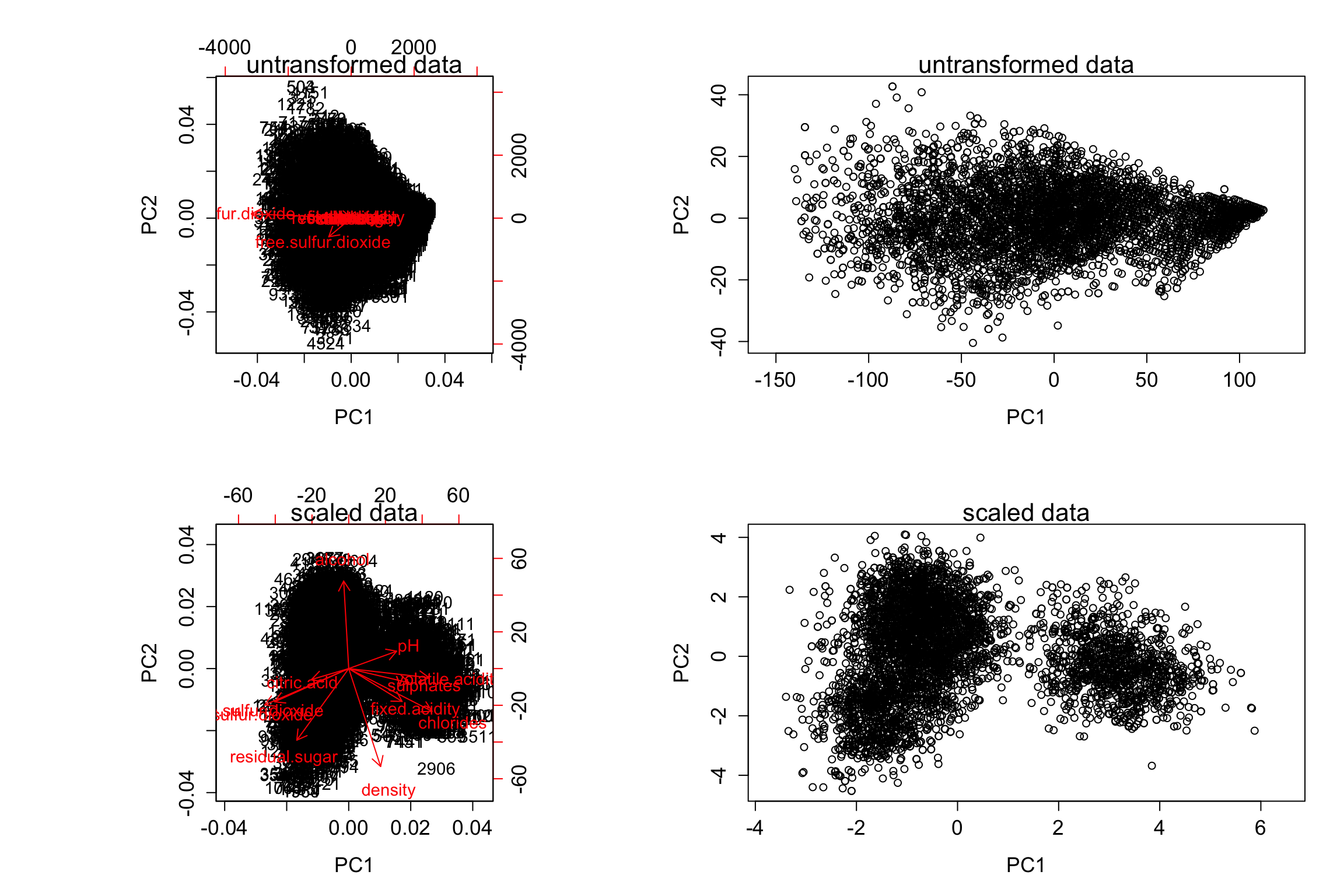
## Ten largest by absolute value loadings, scaled data -- PC1:
## total.sulfur.dioxide            chlorides     volatile.acidity
##           -0.4207814            0.4172822            0.4025068
##  free.sulfur.dioxide            sulphates        fixed.acidity
##           -0.3710354            0.3027714            0.2673589
##       residual.sugar                   pH          citric.acid
##           -0.2599425            0.2402709           -0.1857009
##              density
##            0.1598898
## Ten largest by absolute value loadings, scaled data -- PC2:
##              density              alcohol       residual.sugar
##          -0.58081693           0.51938791          -0.42476884
##            chlorides total.sulfur.dioxide  free.sulfur.dioxide
##          -0.25346298          -0.21569599          -0.19716372
##        fixed.acidity                   pH            sulphates
##          -0.19481681           0.10332072          -0.08433094
##          citric.acid
##          -0.06446984
## PVE by first five PCs (scaled data):
## 32.42024 23.09982 13.69431 8.490649 5.56921par(old.par)
On the scaled version, we can clearly see two clusters.
pcaResTmp = prcomp(mergedWine[, -c(12, 13)], scale.= T)

old.par = par(mfrow=c(1,2))

plot(pcaResTmp$x[, 1:2], xlim = range(pcaResTmp$x[, 1])*1.1, col = mergedWine$quality, main = "Scaled - Display quality")
legend(5.07, 4.44, legend=unique(mergedWine$quality), col=unique(mergedWine$quality), lty=1:2, cex=0.8)

plot(pcaResTmp$x[, 1:2], xlim = range(pcaResTmp$x[, 1])*1.1, col = mergedWine$color, main = "Scaled - Display color")
legend(4.29, 4.44, legend=c("White", "Red"), col=c("grey", "red"), lty=1:2, cex=0.8)
par(old.par)
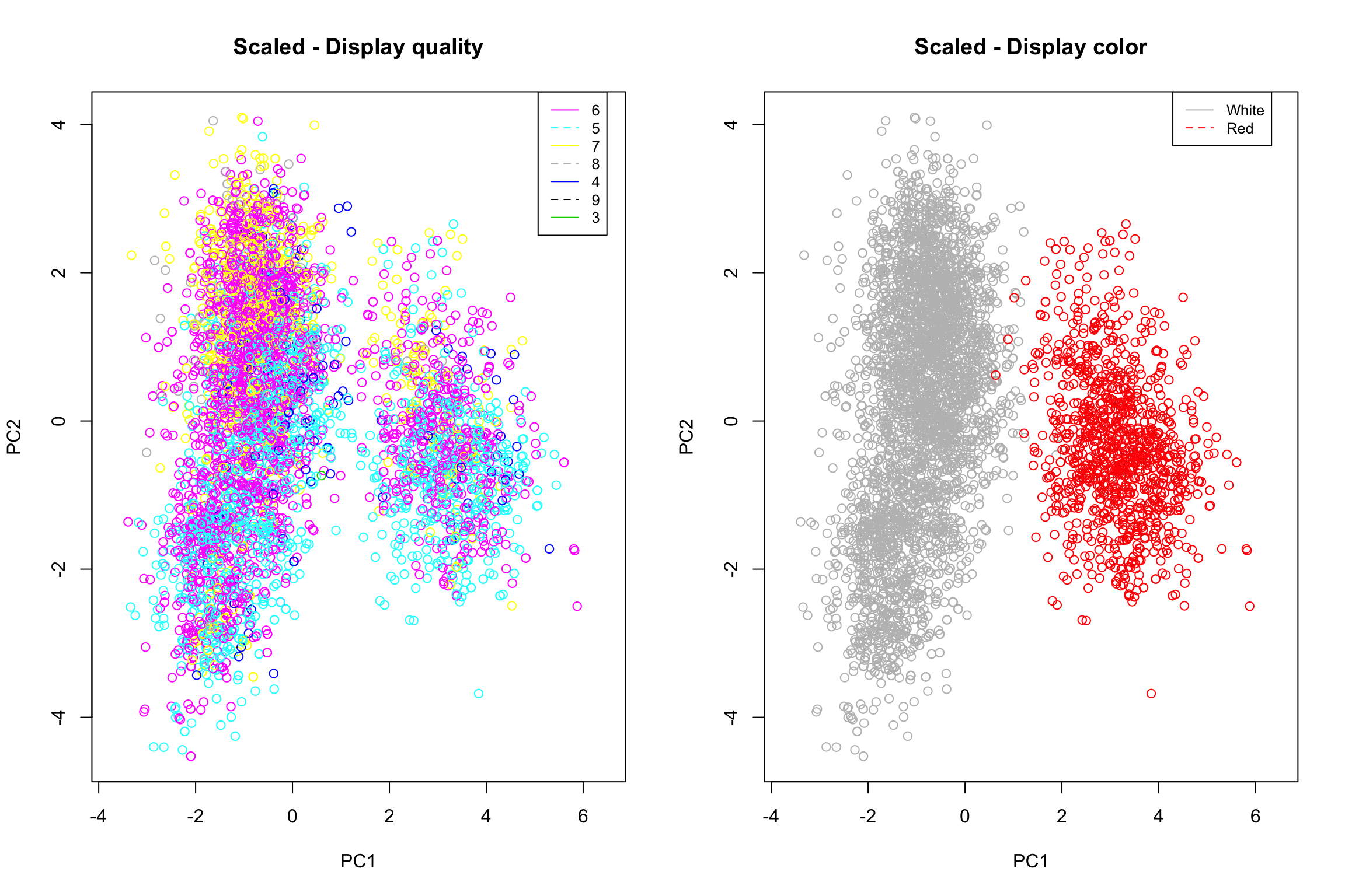
On the first plot we can observe the repartition of the wine quality. There is no “strong” trend but it appears that observations of quality 6 are spread everywhere while observations of quality 7 and 8 tends to be located at the top of each clusters and observations of quality 5 to the bottom.
The second plot show us the wine color repartition. Clearly, the two clusters identified above represent white and red wine, respectively located to the left and the right.
6: Model wine quality using principal components
Compute PCA representation of the data for one of the wine types (red or white) excluding wine quality attribute (of course!). Use resulting principal components (slot x in the output of prcomp) as new predictors to fit a linear model of wine quality as a function of these predictors. Compare resulting fit (in terms of MSE, r-squared, etc.) to those obtained above. Comment on the differences and similarities between these fits.
pcaRed = prcomp(cleanRedDat[, -c(12, 13)], scale.= T)

fit = lm(cleanRedDat$quality~pcaRed$x[,1]+pcaRed$x[,2]+pcaRed$x[,3]+pcaRed$x[,4]+pcaRed$x[,5]+pcaRed$x[,6]+pcaRed$x[,7]+pcaRed$x[,8]+pcaRed$x[,9]+pcaRed$x[,10]+pcaRed$x[,11])
summary(fit)
##
## Call:
## lm(formula = cleanRedDat$quality ~ pcaRed$x[, 1] + pcaRed$x[,
##     2] + pcaRed$x[, 3] + pcaRed$x[, 4] + pcaRed$x[, 5] + pcaRed$x[,
##     6] + pcaRed$x[, 7] + pcaRed$x[, 8] + pcaRed$x[, 9] + pcaRed$x[,
##     10] + pcaRed$x[, 11])
##
## Residuals:
##      Min       1Q   Median       3Q      Max
## -1.92124 -0.36701 -0.05888  0.40757  1.87569
##
## Coefficients:
##                 Estimate Std. Error t value Pr(>|t|)
## (Intercept)     5.645462   0.016751 337.018  < 2e-16 ***
## pcaRed$x[, 1]   0.048462   0.009749   4.971 7.66e-07 ***
## pcaRed$x[, 2]  -0.262717   0.011270 -23.311  < 2e-16 ***
## pcaRed$x[, 3]  -0.124273   0.013202  -9.413  < 2e-16 ***
## pcaRed$x[, 4]   0.101262   0.016228   6.240 6.11e-10 ***
## pcaRed$x[, 5]  -0.012832   0.017991  -0.713  0.47582
## pcaRed$x[, 6]   0.050962   0.020192   2.524  0.01174 *
## pcaRed$x[, 7]   0.134745   0.021044   6.403 2.20e-10 ***
## pcaRed$x[, 8]  -0.001788   0.027009  -0.066  0.94722
## pcaRed$x[, 9]   0.079421   0.028696   2.768  0.00573 **
## pcaRed$x[, 10] -0.114098   0.039794  -2.867  0.00421 **
## pcaRed$x[, 11]  0.081291   0.067025   1.213  0.22543
## ---
## Signif. codes:  0 '***' 0.001 '**' 0.01 '*' 0.05 '.' 0.1 ' ' 1
##
## Residual standard error: 0.5752 on 1167 degrees of freedom
## Multiple R-squared:  0.3947, Adjusted R-squared:  0.389
## F-statistic: 69.17 on 11 and 1167 DF,  p-value: < 2.2e-16
# Calculate the MSE
mean(fit$residuals^2)
## [1] 0.3274646- PC1, PC2, PC3, PC4 and 7 are the important predictors.
- PC5, PC8 and PC11 are not required to explain the variability in quality.
- Adjusted R2 = 0.389 (0.2508 in the previous section).
- MSE = 0.3274646 which is much better than the MSE of the model in the previous section (0.529885).